Decoupled by Design: Billion-Scale Vector Search

Introduction

Vector search has become foundational infrastructure for AI applications — from in-product search to recommendation systems to entity resolution to retrieval-augmented generation. But as datasets grow from millions to billions of vectors, the systems built to serve them start breaking in expensive ways: memory costs explode, ingestion stalls serving, and scaling requires replicating everything.

At Databricks, we ran into these limits with our original vector search offering — so we went back to first principles and redesigned it from scratch. Today, Databricks Vector Search offers two deployment options: Standard endpoints, which keep full-precision vectors entirely in memory for tens-of-milliseconds latency, and Storage Optimized endpoints, which separate storage from compute to serve billions of vectors at a fraction of the cost — with query latencies in the hundreds of milliseconds, a deliberate trade-off for workloads where cost and scale matter more than low-millisecond response times.

Storage Optimized Vector Search was shaped by three core engineering decisions:

1. Separate storage from compute. Vector indexes live in cloud object storage and are loaded into memory only for serving. Ingestion runs on ephemeral serverless Spark clusters, completely isolated from the query path.
2. Build distributed indexing algorithms on Spark. Rather than relying on single-machine indexing libraries, we developed our own — distributed clustering, vector compression, and partition-aligned data layout — as native Spark jobs that scale linearly with cluster size.
3. Serve queries from a Rust engine with a dual-runtime architecture. A purpose-built query engine uses separate thread pools for async I/O and CPU-bound vector computation, so neither starves the other.

The result: billion-vector indexes built in under 8 hours, 20x faster indexing, and up to 7x lower serving costs.

This post is the engineering story of how we built it.

The Problem with Traditional Vector Databases

The Limits of Tight Coupling

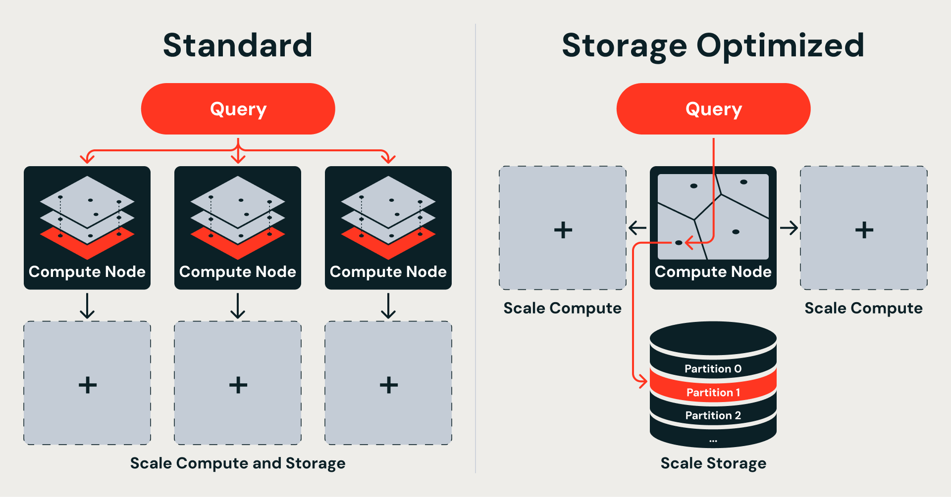
Many production vector databases — including our Standard Vector Search — follow a shared-nothing architecture borrowed from distributed keyword search. Each node owns a random shard of the dataset and maintains an independent in-memory HNSW (Hierarchical Navigable Small World) graph over full-precision vectors. HNSW delivers excellent search quality, but the graph itself must reside entirely in memory, making it one of the most expensive components to scale. This design delivers low latency and supports transactional updates. It works well up to hundreds of millions of vectors.

At billions, it falls apart.

The core issue is coupling. The index, the raw data, and the compute that serves them are all bound to the same node. Scaling means replicating everything: more vectors require more memory, which requires more nodes, each carrying a full copy of its shard's index and data. There is no way to scale storage independently of compute.

The coupling extends to ingestion. Index building happens inside the search engine itself — the same compute resources that handle queries also handle data reorganization, index rebuilds, and compaction. Under write-heavy workloads, query latency degrades. Under query-heavy workloads, ingestion slows to a crawl. Worse, every data change — an upsert, a delete, a compaction — triggers sub-index rebuilds, burning CPU cycles on maintenance rather than serving queries.

Memory-Resident Indexes Are Expensive

That in-memory residency is what makes the architecture fast — and what makes it expensive. At 768 dimensions with 32-bit floats, 100 million vectors consume roughly 286 GiB of RAM, just for the vectors, before any index overhead. A billion vectors would require terabytes. Unlike disk or object storage, where cost per gigabyte is negligible, memory is the most expensive resource in the stack. Every vector added increases the RAM bill directly.

Random sharding compounds the problem. Because vectors are distributed without regard to semantic similarity, every query must scatter to all shards and gather results, regardless of how relevant each shard is. CPU, network overhead, and tail latency all grow with the shard count. Adding vectors means adding shards, and every new shard carries its own memory-resident index.

Decoupled by Design

The answer is not to optimize within this architecture — it is to break the coupling itself.

Storage Optimized Vector Search starts from a single premise: all data lives in cloud object storage, and query nodes are stateless. This splits the system along two boundaries — storage from compute, so query nodes don't own data; ingestion from serving, so index builds never compete with live queries — and gives rise to a three-layer architecture:

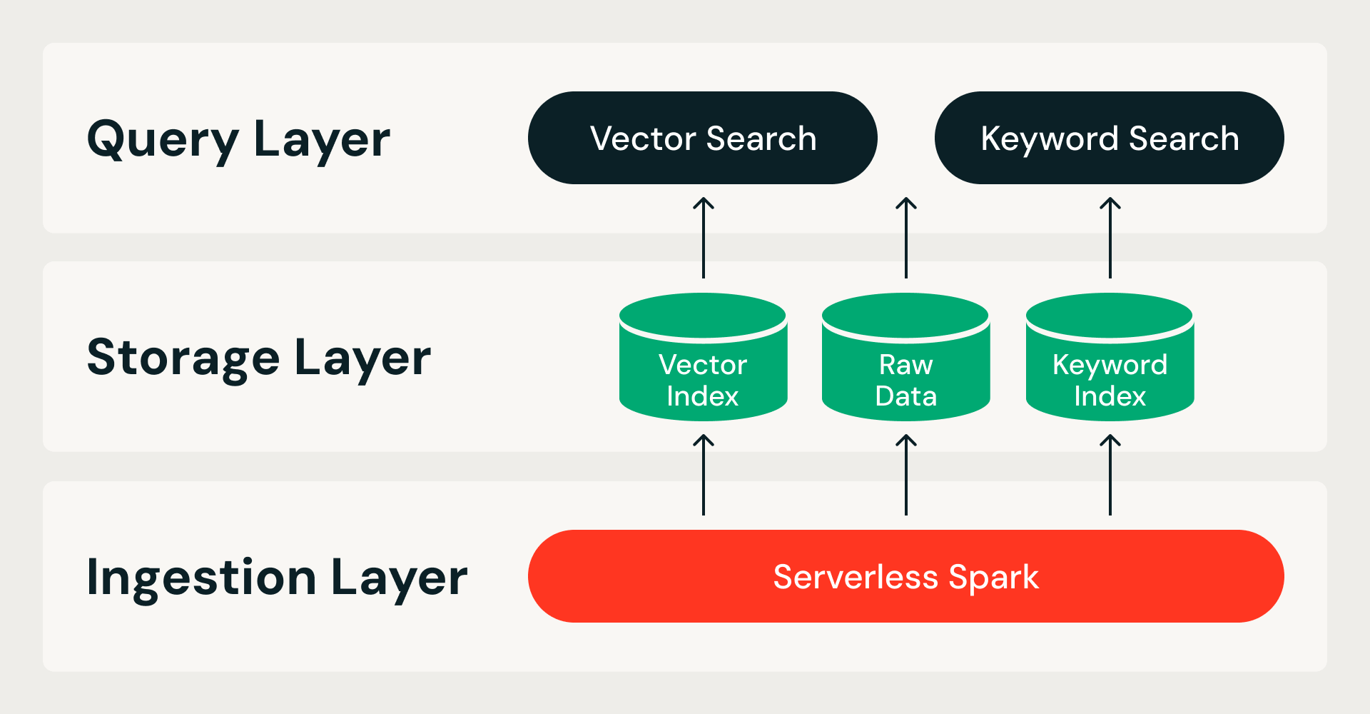
• Ingestion layer. A distributed pipeline on Serverless Spark handles all index building, from raw data to finished index. Each run is idempotent and retriable.
• Storage layer. A custom, cloud-native storage format serves as the system of record. It combines a columnar file format for raw data and vector indexes with an inverted index format for keyword search — all under ACID transactions with immutable data fragments.
• Query layer. Two stateless services handle reads. The vector search service holds a compressed index in memory and fetches full-precision data from object storage on demand. The keyword search serves inverted indexes for metadata filtering and keyword search. Both services scale independently, so resources can be tuned to match the workload.

An Index Structure for Object Storage

If data lives in object storage, the index must be partitionable — the query engine needs to fetch only the relevant slices, not load the entire structure into memory.

HNSW graphs don't have that property. Each search hop can jump anywhere in the graph, so the full structure must be memory-resident to serve a single query. There is no natural way to split an HNSW graph into fragments that map to object storage files.

IVF (Inverted File Index) takes a different approach: it clusters vectors by proximity around learned centroids and searches only the nearest clusters at query time. Each cluster maps directly to a data fragment on object storage — fetchable independently, without loading the rest of the index.

This algorithm choice follows directly from where the data lives. Standard Vector Search keeps the full index in memory for speed, which ties storage and compute together. Storage Optimized moves data to object storage for scale, which frees them — but requires an index that decomposes into self-contained, fetchable partitions. IVF provides exactly that:

Distributed Vector Indexing on Spark

IVF gives us the right index structure for separated storage. The engineering challenge is building it at scale. Most vector indexing libraries — FAISS, ScaNN, Annoy — assume all your data fits on a single machine. That works at tens of millions of vectors. At a billion vectors with 768-dimensional embeddings, you are looking at terabytes of raw floating-point data before you even start building an index. No single machine handles that gracefully, and even if it did, your ingestion time becomes a serial bottleneck that grows with every new row.

We needed indexing that scales horizontally. So we implemented every indexing algorithm from scratch — distributed K-means, Product Quantization, and partition-aligned data layout — as native PySpark jobs running on ephemeral serverless Spark clusters. No single-machine indexing libraries in the critical path. Adding more executors linearly reduces time for the most expensive steps.

The Ingestion Pipeline

Each ingestion run executes as a directed acyclic graph of stages, wrapped in an ACID transaction.

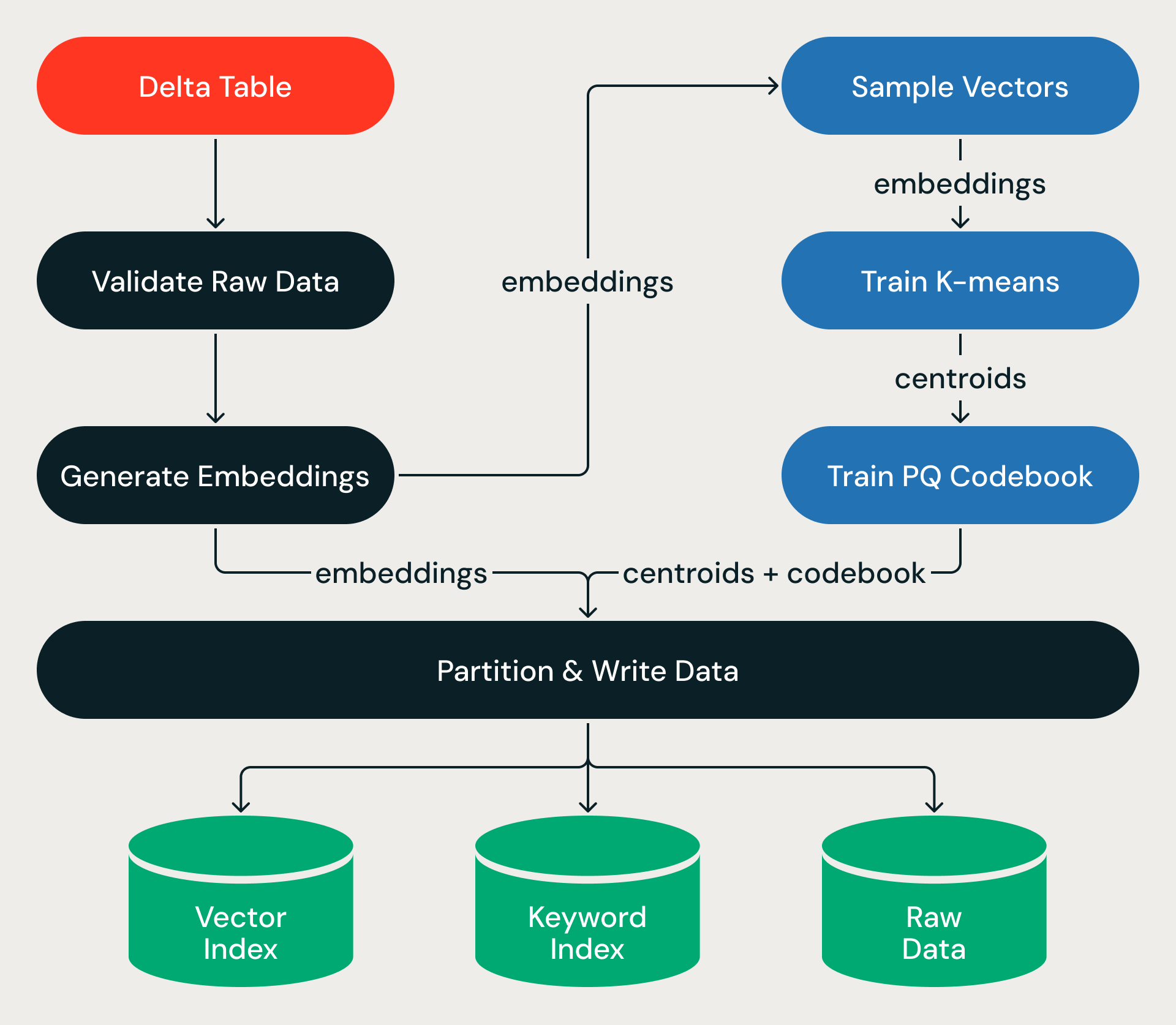
The pipeline starts from a source Delta Table. For indexes backed by source text (rather than pre-computed vectors), after validating the source data, the pipeline calls Mosaic AI Model Serving to generate vector embeddings for new or updated rows — turning billions of text records into high-dimensional vectors at massive scale.

From there, the pipeline trains on a small sample — learning the structure of the vector space — then applies that structure to the full dataset, assigning every vector to a partition, compressing it, and writing the results to object storage. Training is cheap; the full-dataset pass, which shuffles terabytes of data across executors, is where the wall-clock time goes.

K-means: Partitioning at Scale

K-means clustering partitions the vector space into regions — the IVF partitions that let queries search a fraction of the data instead of all of it. For a billion-row dataset, we create roughly 32K partitions. The question is: how do you run K-means at this scale when the standard implementations assume all data fits on a single machine?

You build it from scratch on Spark.

Our implementation uses a hybrid model: Spark handles distributed data movement, while JAX — a numerical computing library with hardware-accelerated linear algebra — handles the math inside each executor. Each K-means iteration is a three-step Spark pipeline:

1. Assign — each executor computes distances from its local batch of vectors to all current centroids, finding each vector's nearest cluster.
2. Shuffle — Spark repartitions the data by centroid ID, co-locating all vectors assigned to the same cluster.
3. Aggregate — each executor computes new centroid positions from its co-located vectors.

The distance computation is the hot loop. JAX compiles it into a single batched matrix operation per executor — computing the full batch-by-centroid distance matrix at once rather than iterating over individual vectors.

Training runs on a sample, not the full dataset — for a billion rows, roughly 8 million vectors (~0.8% of the data). This is not arbitrary: K-means cost per iteration is O(n × k × d), where n is the sample size, k the number of clusters, and d the dimension. Setting both n and k proportional to √N makes total training cost O(N × d) — linear in dataset size regardless of scale.

This choice is also statistically well-founded: coreset theory shows that O(k) samples suffice for high-quality k-means clustering on well-distributed data, and since k scales with √N, our sample size is provably adequate. Training completes in a handful of iterations and checkpoints centroids to object storage for the downstream pipeline stages.

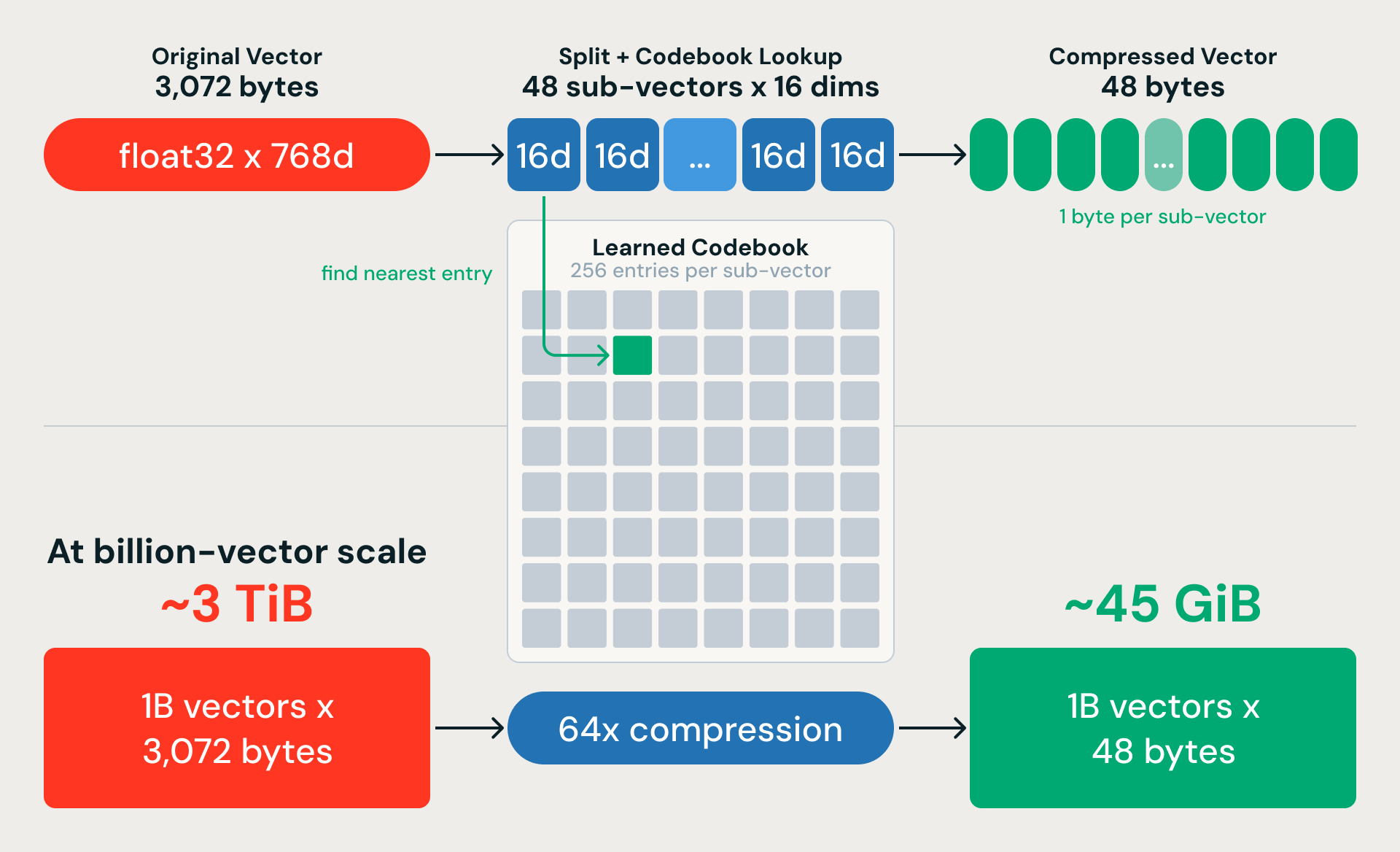
Product Quantization: 64x Memory Compression

K-means gives us coarse partitions. Product Quantization (PQ) compresses the vectors so we can actually search within them at scale. The idea: split each 768-dimensional vector into 48 sub-vectors of 16 dimensions each, and replace each sub-vector with a single byte pointing to the nearest entry in a learned codebook. A 3,072-byte vector becomes 48 bytes — a 64x compression ratio. For a billion 768-dimensional vectors, that shrinks nearly 3 TiB of raw data down to about 45 GiB.

The compression is lossy, but a key design choice recovers most of the accuracy: we train PQ on residual vectors (the difference between each embedding and its nearest K-means centroid) rather than the raw embeddings. K-means captures the large-scale structure; PQ only needs to encode the fine-grained variation within each partition.

From Training to Storage

With centroids and PQ codebooks trained on the sample, the pipeline now processes every row — assigning each vector a partition ID (its nearest centroid) and a compressed PQ code. For a billion-row dataset, this is the most data-intensive stage of the pipeline — a full-dataset Spark job computing distances and encodings across every executor.

Then comes the shuffle. The pipeline repartitions the entire dataset by partition ID, physically co-locating vectors from the same IVF partition in the same data fragments on object storage. This is expensive — terabytes of data move across executors — but it is what makes queries fast. Without co-location, probing a single IVF partition would scatter reads across thousands of files. With it, the same probe hits a handful of contiguous fragments.

The write produces three outputs, each optimized for a different query path:

• Vector Index — compressed PQ codes and partition metadata, written in a format the query engine loads into memory for fast ANN search.
• Keyword Index — inverted index files for metadata filtering and hybrid keyword search.
• Raw Data — full-precision embeddings stored in a columnar format optimized for both sequential scans and random access, fetched on demand during re-ranking.

All three are written as immutable fragments — once written, never modified. When the write completes, a version manifest atomically publishes the new index. This is the contract between ingestion and serving: a set of immutable, partition-aligned data fragments on object storage, ready for the query engine to read directly.

Ingestion at Scale

Storage Optimized supports indexes of over one billion vectors at 768 dimensions — a step change from Standard Vector Search, which caps at 320 million vectors.

Because ingestion runs on ephemeral Spark clusters, fully decoupled from serving, scaling is a matter of adding executors. In practice, this translates to order-of-magnitude improvements across production index builds:

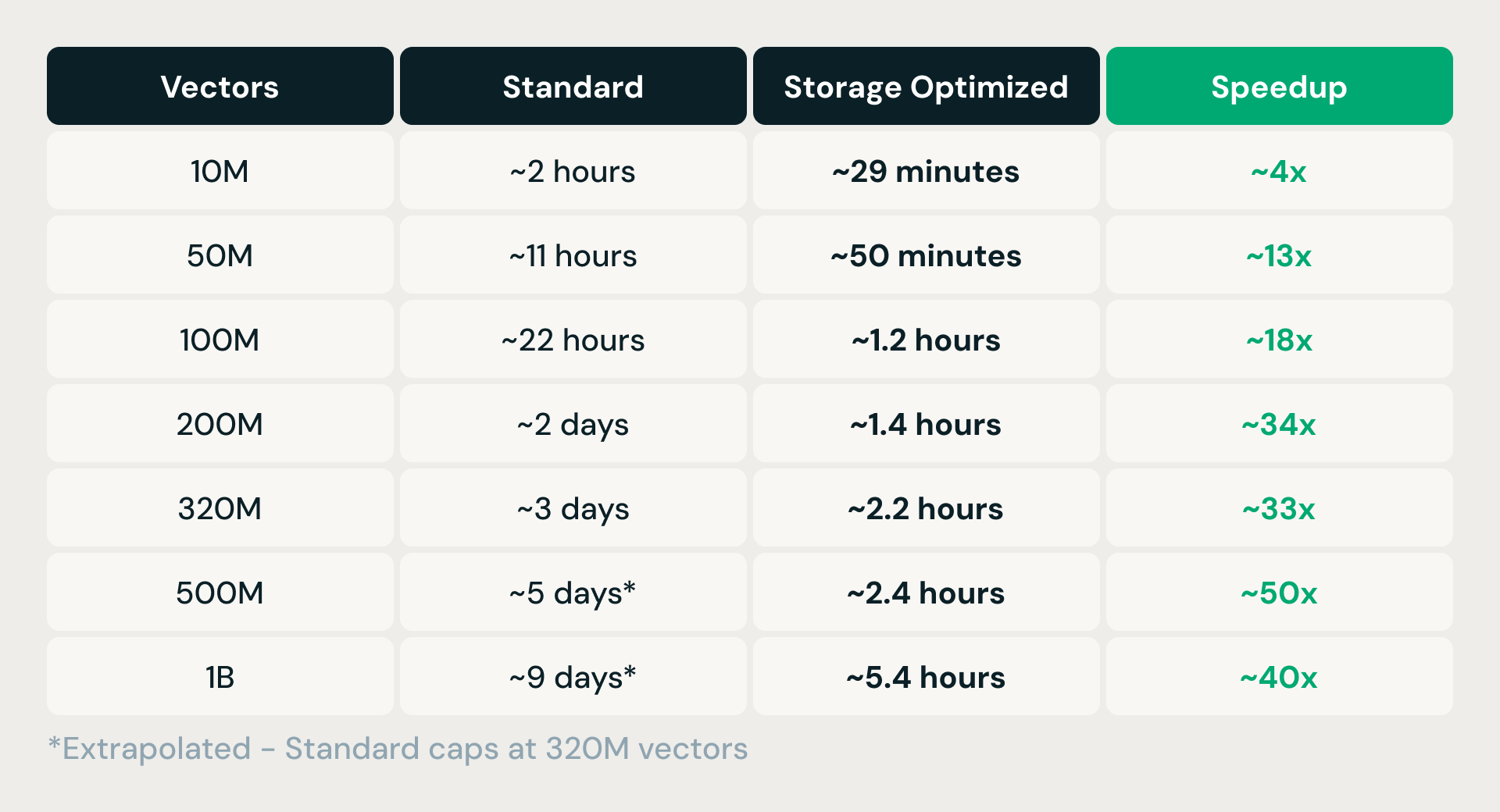
With the index written and atomically published to object storage, the next question is: how do you serve queries against it fast enough for production?

A Query Engine for Object Storage

Separating storage from compute solves the cost problem. But it introduces a new one: every query now involves network round-trips to object storage. The compressed index — small enough to fit in memory — is loaded at startup, but full-precision embeddings stay in blob storage and are fetched on demand or served from a local disk cache. The serving layer has to be fast enough that moving data off-node doesn't compromise query latency.

Anatomy of a Query

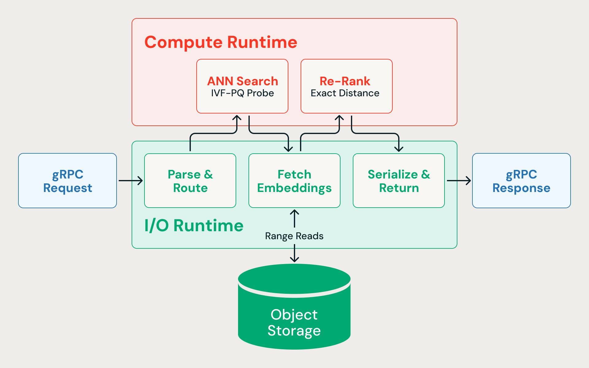
Here is what happens when a nearest-neighbor search hits the engine:

1. Parse & route (I/O). The gRPC request arrives on the async I/O runtime, is deserialized, and routed to the correct index.
2. ANN search (CPU). The query vector is compared against IVF cluster centroids to identify the most relevant partitions. Only those partitions are probed, scanning compressed vectors to compute approximate distances. The search deliberately overfetches candidates — for example, fetching 400 when the caller requests 10 — because quantized distances are approximate and a wider initial net improves final recall after re-ranking.
3. Fetch full-precision vectors (I/O). Concurrent byte-range reads fetch the raw embeddings for each candidate from cloud storage. Because the ingestion pipeline co-locates rows from the same IVF partition in the same data fragment, these reads are partition-pruned — hitting a small number of files, not random-accessing the entire dataset. This step dominates end-to-end latency.
4. Re-rank (CPU). The full-precision embeddings are scored using exact distance computation, recovering the accuracy lost to compression.
5. Serialize & return (I/O). The final top-N results are serialized with their associated metadata and sent back to the caller.

Every query alternates between async I/O and CPU-bound computation. If distance calculations block the async runtime, pending storage reads pile up and latency spikes.

Two Runtimes

The solution is to never let them compete for the same threads. The query engine — written in Rust for predictable latency without GC pauses — splits execution across two dedicated thread pools: one for async I/O, one for CPU-bound vector math. Neither workload can starve the other.

The I/O runtime runs on the Tokio async executor and handles gRPC request parsing, blob storage range reads, inter-service communication, and response serialization. Because storage reads are the latency bottleneck, this runtime needs to keep hundreds of concurrent requests in flight without blocking.

The compute runtime runs vector distance calculations, partition probing, and re-ranking on its own pool of threads. A subset of CPU cores is explicitly reserved for the I/O runtime — compute is never allowed to consume the entire machine.

Read Coalescing

Beyond thread isolation, the I/O path itself required tuning. Early profiling revealed that the engine was issuing many small, single-vector range reads to object storage. Each call carries per-request overhead and latency variability — with long tails reaching hundreds of milliseconds — so many tiny requests meant high per-query latency variance.

The fix was read coalescing: instead of issuing one range read per vector, the storage layer sorts pending byte-range requests by file offset and merges any that fall within a configurable block-size window into a single read. Fewer, larger requests means less per-call overhead, but each merged read also fetches bytes the query doesn't need — read amplification. The trade-off required empirical tuning.

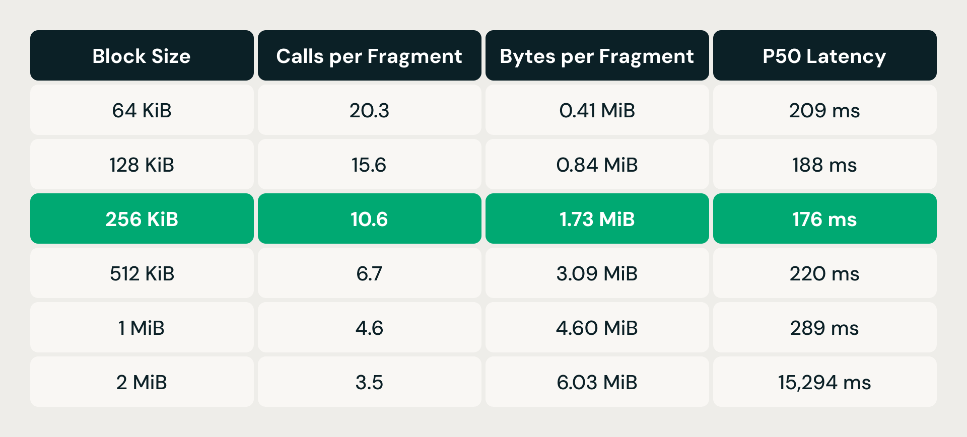
At 64 KiB, each data fragment required over 20 storage calls but fetched less than half a megabyte — per-request overhead dominated. Doubling the block size steadily reduced call counts, and latency improved through 256 KiB. But past that point, read amplification took over: at 512 KiB, latency climbed back above the 64 KiB baseline despite far fewer calls. At 2 MiB it exploded to over 15 seconds. The 256 KiB sweet spot cut calls roughly in half while keeping read amplification under 2 MiB per fragment, delivering the lowest p50 latency of any configuration tested.

Putting It All Together

Everything in this architecture trades query latency for scale and cost. At 768 dimensions and top-10 results, recall — the fraction of true nearest neighbors returned — stays above 94% at 10 million vectors, above 91% at 100 million, and holds at 90% even at a billion: the reranking step, which fetches full-precision vectors from object storage and recomputes exact distances, recovers accuracy that compressed codes alone would lose at scale. That reranking round-trip is also what dominates query time — queries return in about 300 milliseconds at 10M vectors and roughly 500 milliseconds at a billion, compared to 20–50 milliseconds on Standard endpoints, which keep everything in memory.

What you get for those extra milliseconds: index builds at billion-vector scale complete in under 8 hours, 20x faster than Standard on large datasets. Product Quantization compresses the in-memory footprint by more than an order of magnitude, ingestion runs on ephemeral Spark clusters that release resources after each build, and decoupling storage from serving means neither side is over-provisioned. The result is up to 7x lower cost for customers at the same scale.

For many workloads — semantic search, recommendation pipelines, retrieval-augmented generation — that trade clearly favors scale and cost. Post-retrieval stages (ranking, filtering, LLM generation) often dominate end-to-end time, making the difference between 40 and 400 milliseconds invisible to the end user. For latency-sensitive serving where every millisecond matters, Standard Vector Search remains the better tool. The two options are complementary — different tools for different workloads.

What We Learned

Building a vector search system from scratch — rather than optimizing the one we had — forced a set of bets that only pay off in combination.

Storage-compute separation only works if the query engine is fast enough. Moving data off-node saves money, but it adds I/O to every query — whether that is network round-trips to object storage or reads from a local disk cache. The dual-runtime Rust engine exists specifically to absorb that latency: async I/O keeps hundreds of reads in flight while CPU threads handle distance computation without blocking. Without that engine, the architecture would deliver cheap storage and slow queries — not a compelling trade-off.

Distributed indexing only works if the index format supports it. Building K-means and PQ on Spark gives us horizontal scale for ingestion, but the output has to be something the query engine can serve directly from object storage without a rebuild step. The custom storage format — immutable data fragments, separated transaction manifests, ACID semantics on cloud storage — closes that loop. Ingestion writes directly to the format the query engine reads.

Compression is the economic lever. Product Quantization does not just reduce memory cost. It changes the architecture's viability. Without this level of compression, storing quantized codes in memory for a billion vectors would still require terabytes of RAM, and the cost advantage over Standard Vector Search would evaporate. PQ makes it possible to keep the ANN search phase in memory while pushing everything else to object storage.

These are not independent optimizations. Remove any one, and the system either costs too much, builds too slowly, or serves too slowly to be practical.

Conclusion

The hard problems ahead follow directly from these trade-offs. Pushing query performance further — faster responses, higher throughput, better concurrency — through smarter caching, tiered storage, and denser in-memory representations. Making updates near-real-time at billion scale. Moving beyond raw vector distance as the final ranking signal — toward learned, multi-stage ranking that combines vector similarity, keyword relevance, and domain context into results that are not just nearest, but most useful.

We believe the next generation of AI products will be built on infrastructure that hasn't been invented yet — and that the engineers who build that infrastructure will shape what AI can do. If you want to be one of them, come build with us!