Efficiently Estimating Pareto Frontiers with Cyclic Learning Rate Schedules

Benchmarking the tradeoff between model accuracy and training time is computationally expensive. Cyclic learning rate schedules can construct a tradeoff curve in a single training run. These cyclic tradeoff curves can be used to evaluate the effects of algorithmic choices on network training efficiency.

This work is has been posted as an arXiv preprint: Fast Benchmarking of Accuracy vs. Training Time with Cyclic Learning Rates.

Problem Statement: Producing Tradeoff Curves Efficiently

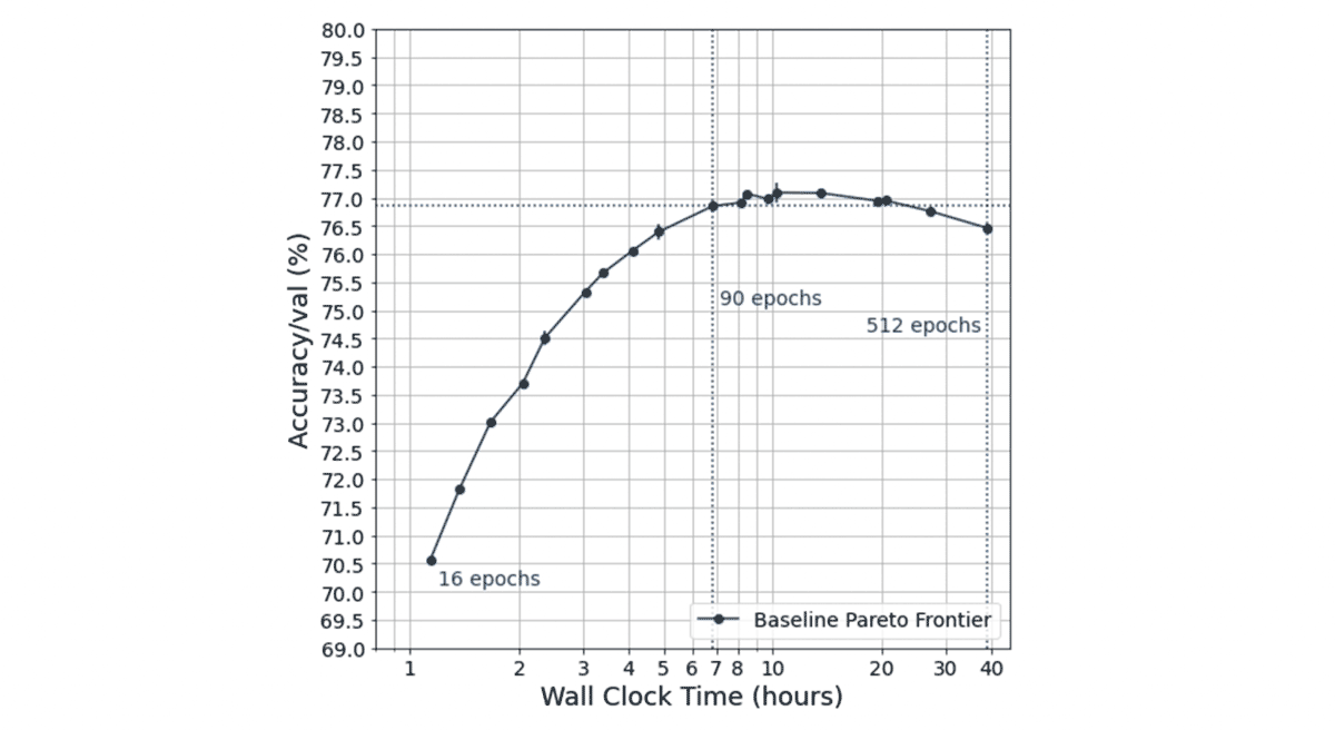
At MosaicML, we design changes to the neural network training algorithm (which we call speedup methods) that lead to better tradeoffs between the cost of training a model and the quality of the trained model. We evaluate the efficacy of these interventions by looking at the tradeoff between training time and model quality. Concretely, we look at tradeoff curves like the one below.

With this as background, our problem statement is as follows: Given a fixed recipe for training (e.g. architecture, objective function, regularization methods), how can we efficiently produce a tradeoff curve?

One approach might be to sparsely sample points across different possible training durations and then interpolate. For example, we could train a network for three different durations (e.g. 30, 90, 270 epochs on an exponential scale) and fit a parameterized function to interpolate the rest of the curve. In this scenario, training would take 390 epochs total. We use this approach extensively in our MosaicML Explorer benchmarking across cloud instances, hardware choices, and speedup methods. However, the added expense of doing so was especially painful given that we performed thousands of training runs to collect this data. For the remainder of the blog, we refer to any tradeoff curve generated this way as the standard tradeoff curve.

Another approach might be to do one long training run (e.g. for 270 epochs) and sample points on the tradeoff curve during training. However, modern training best-practices involve gradually decaying the learning rate over the course of training. Many of the points sampled in this procedure will therefore be at intermediate states where training is not complete and the learning rate schedule is atypically high, leading to lower-than-normal model quality.

Neither of these approaches is satisfactory. The first approach is too computationally expensive, and the second produces low-fidelity results that are not indicative of standard performance.

The Solution: Cyclic Learning Rates

In this blog post, we show that multiplicative cyclic learning rate schedules can be used to construct an accuracy-time tradeoff curve in linear time, i.e., in a single training run, saving time and money. Although using this method necessarily changes the outcome of training, we still find that it provides similar-fidelity information about the relative efficacy of different speedup methods. This is particularly exciting because it means that ML researchers can characterize the accuracy-time tradeoff more efficiently, and therefore make meaningful comparisons between choices of architectures, hyperparameters and network training methods.

We recommend that accuracy-time tradeoff curves should be standard practice for ML research (in addition to accuracy tables!). With cyclic learning rate schedules, generating tradeoff curves is not computationally expensive.

Background: Characterizing Training Performance with Pareto Frontiers

At MosaicML, we care about speeding up neural network training. We have found it particularly useful to frame neural network training as a tradeoff between accuracy and time as depicted in the tradeoff curve below.

We produce tradeoff curves by varying the length of training for each model configuration; longer training runs take more time (further to the right on the x-axis) but tend to reach higher quality (higher on the y-axis). A Pareto frontier is the set of all of the best possible tradeoffs between training time and accuracy, where any further attempt to improve one of these metrics worsens the other. For a fixed model and task configuration, this method of generating tradeoff curves is an estimate of the theoretical Pareto frontier. Constructing a tradeoff curve allows us to then make claims such as:

• For a desired accuracy A, the network need only be trained for a particular amount of time T
• Given a time budget T, accuracy A can be achieved

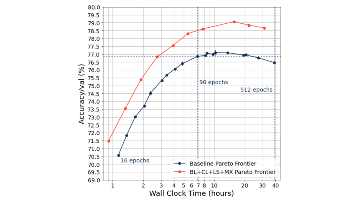
We consider one configuration to be better than another if the tradeoff curve it produces is further upward and to the left (e.g., the orange curve in the figure above). Accuracy-time tradeoff curves also allow us to make quantitative statements about different hyperparameter choices and training algorithms, for example:

• Training the same network with Blurpool (Zhang 2019), Channels Last, Label Smoothing (Szegedy et al. 2015, Müller et al. 2015), and MixUp (Zhang et al. 2017) shifts the tradeoff curve left along the time axis and up along the quality axis, leading to a Pareto improvement in both accuracy and speedup relative to the baseline

Cyclic Learning Rate Schedules

The learning rate at which a neural network is trained is often called “the most important hyperparameter” (Howard and Gugger 2020). In many modern implementations, the learning rate is a scalar value that is first increased with a linear warmup, and then decreased with a cosine decay. Historically (i.e. 5 years ago!), there was a flurry of work exploring alternative learning rate schedules from exponential decays to trapezoids. Cyclic learning rates fall on the more exotic end of the spectrum. [1]

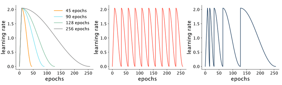
Cyclic learning rate schedules for CIFAR-10 and ImageNet were first proposed in Smith (2015). They essentially increase and decrease the learning rate periodically during training. While Smith (2015) proposed various sawtooth-like schedules, Loshchilov and Hutter (2016) showed that a schedule designed with cycles of a cosine decay followed by a restart led to competitive accuracy on CIFAR-100. The basic (noncyclic) cosine decay schedule also introduced by this paper is widely used today. Some variations of cosine decay with restarts include schedules with a constant period and schedules with periods that increase multiplicatively, which we call multiplicative cyclic learning rate (CLR) schedules. [2]

Cyclic learning rate schedules were popularized by Fast.ai (Howard and Gugger 2020), but are not widely used in the research community. This is likely due to the fact that, with current best practices on benchmarks like ImageNet, cyclic learning rate schedules do not necessarily lead to improved (or even commensurate) accuracy when compared to cosine decay schedules (data not shown). And while some of the early motivation for cyclic learning rates was to be able to interrupt training at any time and still return good performance (a.k.a. an “anytime” algorithm), anytime performance is not necessarily of interest for heavily studied benchmarks with known, standard hyperparameters. However, we suspected that cyclic learning rate schedules could be used to efficiently construct accuracy-time tradeoff curves.

In the rest of this blog post, we show how you can use multiplicative cyclic learning rate (CLR) schedules to efficiently construct useful accuracy-time tradeoff curves for benchmarking ImageNet. We then explore how these curves change for combinations of regularization and speedup methods, such as Blurpool, Channels Last, Label Smoothing, and Mixup. All experiments use ResNet-50 on ImageNet, and report top-1 validation accuracy.

Cyclic Learning Rate Schedules with Constant Period Generate Suboptimal Tradeoff Curves

We first used cyclic learning rate (CLR) schedules with constant periods, and examined the effect of varying the periods (10, 20, 30, 40, and 50 epochs). This led to an interesting trend, whereby cyclic learning rate schedules with shorter periods (e.g. 10 epochs, gray line) led to suboptimal tradeoff curves, while CLRs with longer periods (e.g. 50 epochs, magenta line) led to curves that were on the standard tradeoff curve.

The bottom line: Cyclic learning rate schedules aren’t always good, and high-frequency cycling can lead to poor validation accuracy.

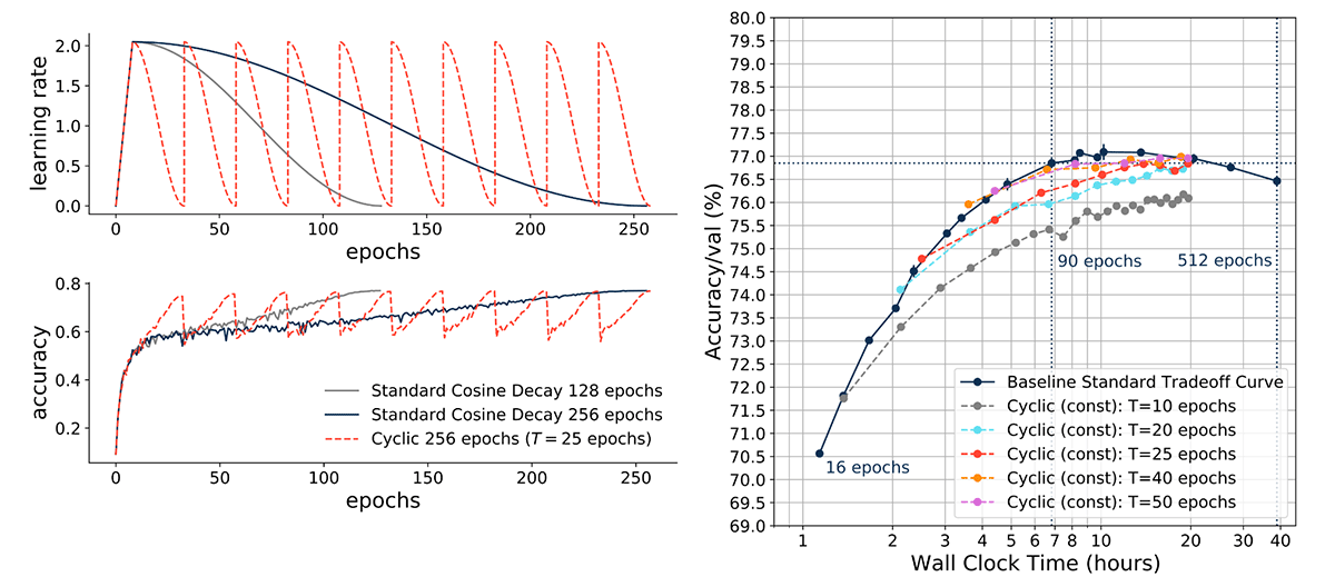
Multiplicative Cyclic Learning Rate Schedules Efficiently Estimate Tradeoff Curves

We then used multiplicative cyclic learning rate schedules with doubling periods, and found that they approximated the baseline standard tradeoff curve quite well. For the rest of this blog post, we refer to these curves as cyclic learning rate (CLR) tradeoff curves.

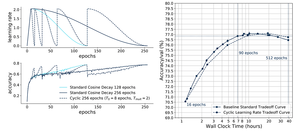
Specifically, we designed the learning rate schedule to linearly warm up for 8 epochs to a maximum value of 2.048, and then cycle with a cosine decay for increasing periods of 8, 16, 32, 64, 128 and 256 epochs, for a total of 512 epochs of training. We then stored maximum accuracy values at the end of each cycle, and plotted an accuracy-time tradeoff curve. This was straightforward to implement in PyTorch with the CosineAnnealingWarmRestarts learning rate scheduler. [3]

This CLR tradeoff curve matched our ResNet-50 ImageNet baseline standard tradeoff curve (with a difference of -0.084% on average across three seeds). This result held across choices of periods (e.g. starting with 5 epochs, then doubling to 10, 20 etc. epochs; data not shown).

The bottom line: Multiplicative cyclic learning rate schedules with doubling periods can be used to construct accuracy-time tradeoff curves.

Cyclic Learning Rate Tradeoff Curves Approximate Pareto Frontiers Across Training Methods

There are a handful of demonstrated methods that modify the training procedure to achieve better tradeoffs between the final model quality and the time or cost to train the model. Some of these methods include Blurpool (Zhang 2019), Channels Last, Label Smoothing (Szegedy et al. 2015, Müller et al. 2015), and MixUp (Zhang et al. 2017). In our benchmarking work for MosaicML Explorer, we wanted to find methods in the literature that led to clear Pareto improvements.

We therefore asked whether multiplicative cyclic learning rate schedules could be used to construct competitive accuracy-time tradeoff curves for separate methods such as Blurpool, Channels Last, Label Smoothing, and MixUp. We found that using multiplicative cyclic learning rate schedules allowed us to generate tradeoff curves of comparable quality to standard tradeoff curves, but at substantial time savings (~2x).

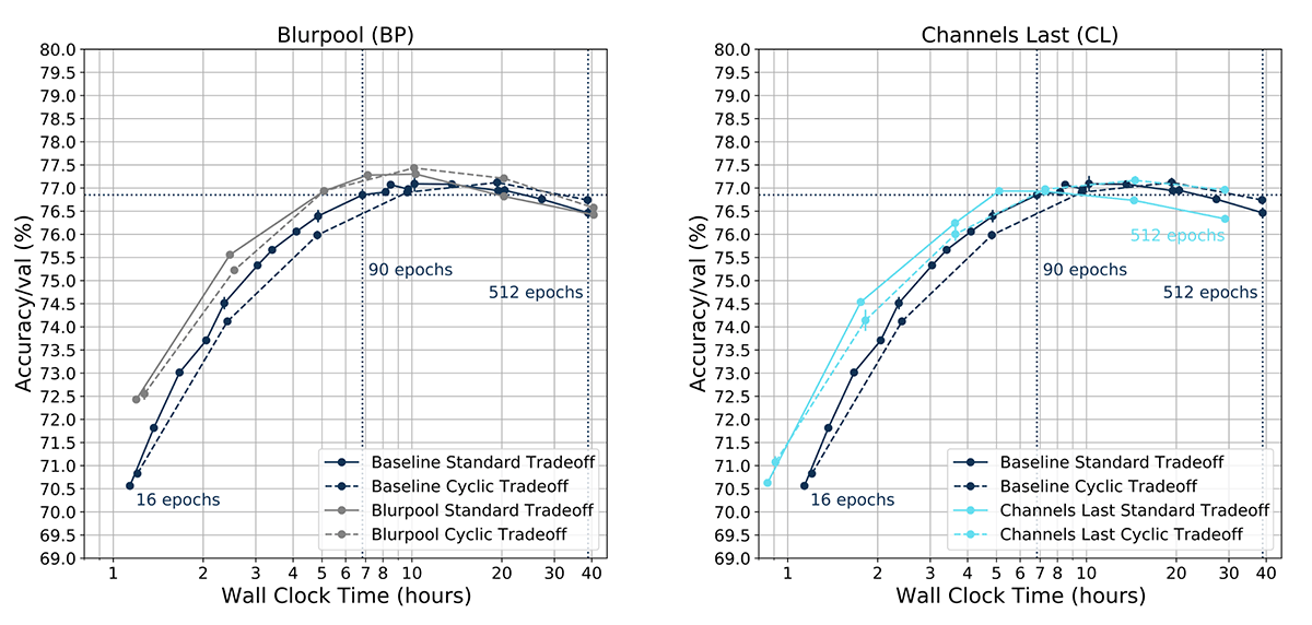
Blurpool, Channels Last

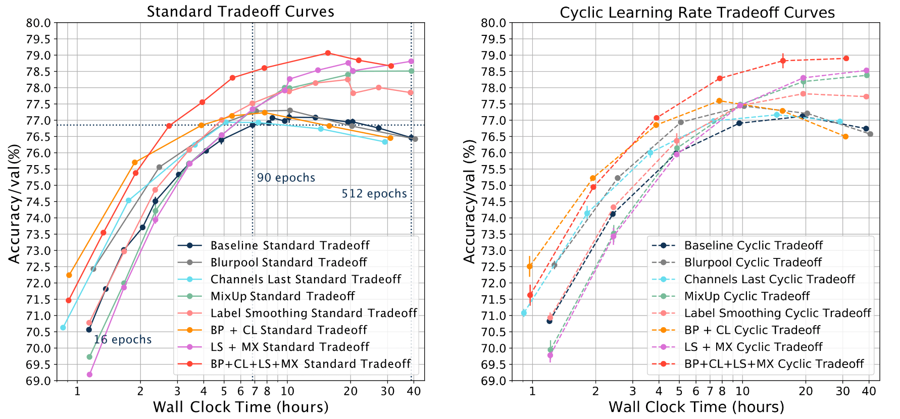
We found that cyclic learning rate tradeoff curves were able to match baseline standard tradeoff curves for Blurpool and Channels Last almost exactly (Blurpool exceeded by 0.07%, and Channels by 0.09%, on average). Note that the simple Channels Last modification on RTX 3080 GPUs led to a leftward shift of the tradeoff curve along the time axis (solid cyan line); thus training a network for 512 epochs took approximately 30 hours instead of 40 hours. Also note that Blurpool led to strong improvements for shorter training times (e.g. 16 epochs).

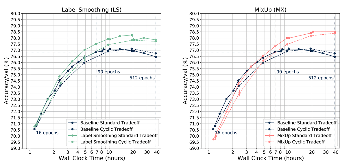
Label Smoothing, Mixup

Cyclic learning rate tradeoff curves were slightly below baseline standard tradeoff curves for Label Smoothing and MixUp, on average differing roughly by -0.44% for Label Smoothing and -0.39% for MixUp. Importantly, CLR tradeoff curves for these two cases still trended with the standard tradeoff curves.

Blurpool + Channels Last, Label Smoothing + MixUp

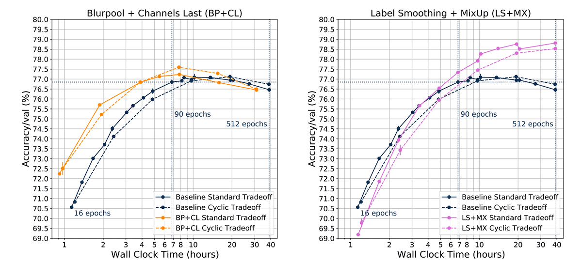
Constructing a separate tradeoff curve for every training method and/or combination of methods (for example Label Smoothing + Mixup) is also combinatorially expensive. We therefore asked whether cyclic learning rate schedules could accurately construct tradeoff curves for combinations of methods. We trained ResNet-50 with both Blurpool and Channels Last (BP + CL), and found that the cyclic learning rate schedule tradeoff curve matched the Pareto frontier for shorter training durations (on average, exceeded by 0.08%). This was not surprising, as the CLR tradeoff curves for Blurpool and Channels Last individually led to improvements with respect to the baseline standard tradeoff curve.

We then trained ResNet-50 with the combined methods of Label Smoothing and MixUp (LS + MX), and found that CLR tradeoff curves trended with standard tradeoff curves, but were slightly lower (by -0.46% on average). This made sense considering the results for Label Smoothing and MixUp individually.

Blurpool + Channels Last + Label Smoothing + MixUp

Finally, we trained ResNet-50 with the combined methods of Blurpool, Channels Last, Label Smoothing and MixUp (BL + CL + LS + MX), and found that CLR tradeoff curves trended with the standard tradeoff curves (crimson dashed line, lower by -0.24% on average).

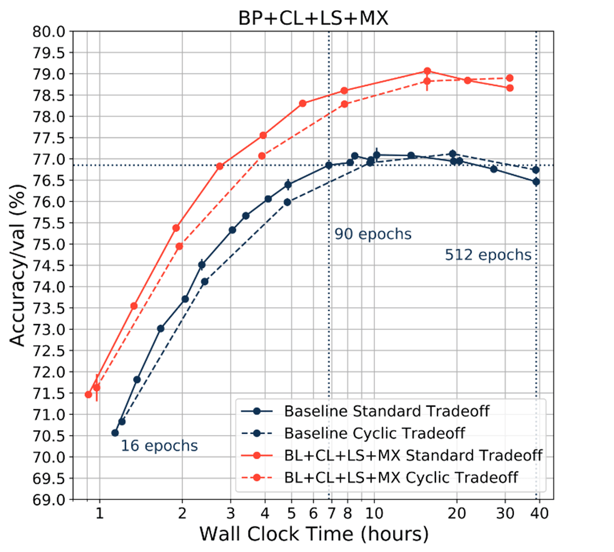
We then plotted the total wall clock time for standard tradeoff curves and cyclic learning rate (CLR) tradeoff curves with six sampled points at 16, 32, 64, 128, 256 and 512 epochs. As expected, standard tradeoff curve total wall clock time was almost twice as long as CLR tradeoff curve total wall clock time across all training methods

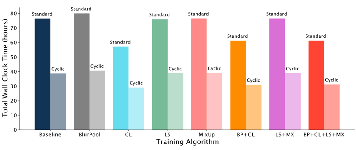
The ratio of the time to construct a standard tradeoff curve versus the time to construct the cyclic tradeoff curve (where both tradeoff curves sample the same exact points) can be expressed in the following formula:

Here a is the starting number of epochs, r is the multiplicative factor, and n-1 is the total number of sampled points. When r=2, this ratio is approximately 2, meaning that using a cyclic learning rate schedule will lead to ~2x speedup.

We also found that CLR tradeoff curves matched relative trends between standard tradeoff curves across training methods. For example, MixUp (MX) has worse accuracy relative to baseline for shorter training times of 16 epochs (<70%), and performs better than Label Smoothing (LS) for longer training times of 512 epochs (above 78.5%).

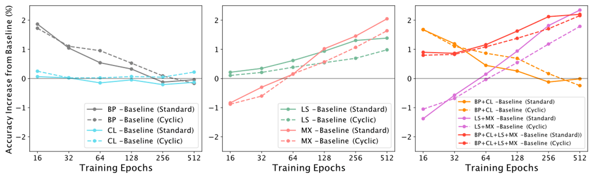
When comparing training methods such as Label Smoothing and MixUp, can we really trust that improvements in the Pareto frontier over the baseline will be matched by a tradeoff curve constructed with a cyclic learning rate? One way to assess this is simply to compare the relative improvements over baseline for each method. When we subtract the Blurpool standard tradeoff curve from the Baseline standard tradeoff curve, we can see that early on in training Blurpool provides a 2% accuracy boost, but provides no accuracy boost at 256 epochs (gray solid line). Subtracting the Blurpool CLR tradeoff curve from the Baseline CLR tradeoff curve shows the same trend (gray dashed line). We can also take the cosine similarity between these two lines. Across the training methods and combinations of training methods, we can see that CLR tradeoff curves match the trends nicely (cosine similarity BP=0.972, CL=-0.273, LS=0.992, MX=0.976, BP+CL=0.952, BP+CL=0.989, BP+CL+LS+MX=0.997).

This is all to say that if a method such as MixUp shifts the standard tradeoff curve, it also correspondingly shifts the CLR tradeoff curve.

The bottom line: Tradeoff curves constructed using multiplicative cyclic learning rate schedules can provide information on the relative performance of speedup methods.

Why This Works

It is somewhat surprising that multiplicative cyclic learning rates are able to approximate Pareto frontiers when constant period cyclic learning rates do not. Why does this work, particularly for increasing periods? One possibility might have to do with different phases of learning (Golatkar et al., 2019, Frankle et al., 2020). For example, rapid changes in learning rate might help find better minima early in training (10-20 epochs), while very slow changes in learning rate might help find minima in already “good” basins late in training (>90 epochs). As training continues, it might become more difficult to find better minima, implying that it might be beneficial to take longer for each new cycle. [4]

We were particularly intrigued by the precipitous changes in accuracy during the learning rate cycles; we found this to be a clear illustration of explore versus exploit dynamics happening across different minima. This has been noted by multiple studies, and is one of the motivating factors for ensembling methods (e.g. Huang et al., 2017) and Stochastic Weight Averaging (SWA, Izmailov et al., 2018).

Future Directions

In many instances, the CLR tradeoff curve underestimated the standard tradeoff curve by a margin of ~0.5% validation accuracy. There are many possible variations to our approach that might improve this gap. Some ideas include:

• Allowing the entire cyclic learning rate schedule to decay over the course of learning. This would mean decreasing the maximum learning rate after each reset. This is one of many schedule variations explored by the literature (Schmidt et al. 2021)
• Applying Stochastic Weight Averaging (SWA, Izmailov et al., 2018) at the end of each cycle. This would entail, at the end of each trough, cycling the learning rate (even more!) at low amplitude and at high frequency, and averaging the weights. Such an approach might boost the validation accuracy and lead to Pareto optimality in some instances. [5]
• Repeating linear warm up instead of a hard reset, although it is unclear if this would improve accuracy. We found that sawtooth/triangular cyclic learning rate schedules did not get close to the Pareto frontier for ResNet-50 on ImageNet (data not shown).
• Experimenting with other multiplier values. The behavior of the PyTorch CosineAnnealingWarmRestarts scheduler makes it difficult to control the spacing of points sampled along the Pareto curve, in part due to the constraint of epoch-wise (and not step-wise) scheduling. We hope to circumvent this problem in future versions of Composer.
• Applying a cyclic learning rate to other hyperparameters such as weight decay, batch size, and gradient clipping (in line with Smith 2022).

Our cyclic learning rate approach to constructing tradeoff curves worked nicely for training methods such as Blurpool and Label Smoothing. However, in the current implementation of MosaicML Composer (or PyTorch), it won’t work for methods that have their own independent schedules such as Layer Freezing (Brock et al., 2017), Stochastic Weight Averaging (SWA) (Izmailov et al., 2018), and Progressive Resizing (Fast.ai). It can work in principle, however, if the schedules for methods such as Progressive Resizing cycle with the learning rate schedule. We hope to implement this in future versions of the library.

The use of Pareto frontiers in ML research is surprisingly limited, and is mostly restricted to the subfield of multi-objective optimization (MOO) for multitask learning (some recent examples include Lin et al., 2020 and Navon et al., 2020). [6] At MosaicML, we have found that thinking about Pareto optimality is useful for framing more fundamental questions in neural network training.

Our results primarily hold for convolutional networks (ResNet-50, ResNet-101) applied to computer vision tasks (CIFAR-10 and ImageNet). Can the same approach be applied to NLP? A lot of the recent scaling law papers find a linear boundary based on single, full training runs, where the scaling is based on model size (Henighan et al., 2020). However, it is likely that each model size has an associated quality-time Pareto frontier. Is it possible to shift the scaling laws to have better exponents? Some of our preliminary experimentation is inconclusive. We hope to explore this in future work.

Takeaways

We have shown here that multiplicative cyclic learning rate schedules can be used to construct an accuracy-time tradeoff curve in a single training run, saving time and money. This is a practical means of assessing changes in tradeoff curves caused by different architectures, hyperparameters, and speedup methods.

We hope that this is a small step towards framing ML efficiency in terms of tradeoff curves and Pareto optimality.

This work was done as part of a research internship with MosaicML. Thanks to Cory Stephenson, Davis Blalock, Kobie Crawford and Jonathan Frankle for fruitful discussions.

References

1. Blalock, D., Ortiz, J. J. G., Frankle, J., & Guttag, J. (2020). What is the state of neural network pruning?. arXiv preprint arXiv:2003.03033.
2. Blalock, D., Carbin, M., Florescu, L., Frankle, J., Leavitt, M., Lee, T., Nadeem, M., Portes, J., Rao, N., Seguin, L., Stephenson, C., Tang, H., Venigalla A., (2021) On Evaluating and Improving the Efficiency of Deep Networks Whitepaper
3. Brock, A., Lim, T., Ritchie, J. M., & Weston, N. (2017). Freezeout: Accelerate training by progressively freezing layers. arXiv preprint arXiv:1706.04983.
4. Fedyunin, V. (2021) Channels Last Memory Format in PyTorch (PyTorch documentation)
5. Frankle, J., Schwab, D. J., & Morcos, A. S. (2020). The early phase of neural network training. arXiv preprint arXiv:2002.10365.
6. Golatkar, A. S., Achille, A., & Soatto, S. (2019). Time matters in regularizing deep networks: Weight decay and data augmentation affect early learning dynamics, matter little near convergence. Advances in Neural Information Processing Systems, 32.
7. Henighan, T., Kaplan, J., Katz, M., Chen, M., Hesse, C., Jackson, J., ... & McCandlish, S. (2020). Scaling laws for autoregressive generative modeling. arXiv preprint arXiv:2010.14701.
8. Howard, J., & Gugger, S. (2020). Fastai: a layered API for deep learning. Information, 11(2), 108.
9. Huang, G., Li, Y., Pleiss, G., Liu, Z., Hopcroft, J. E., & Weinberger, K. Q. (2017). Snapshot ensembles: Train 1, get m for free. arXiv preprint arXiv:1704.00109.
10. Izmailov, P., Podoprikhin, D., Garipov, T., Vetrov, D., & Wilson, A. G. (2018). Averaging weights leads to wider optima and better generalization. arXiv preprint arXiv:1803.05407.
11. Lin, X., Yang, Z., Zhang, Q., & Kwong, S. (2020). Controllable pareto multi-task learning. arXiv preprint arXiv:2010.06313.
12. Loshchilov, I., & Hutter, F. (2016). Sgdr: Stochastic gradient descent with warm restarts. arXiv preprint arXiv:1608.03983.
13. Loshchilov, I., & Hutter, F. (2017). Decoupled weight decay regularization. arXiv preprint arXiv:1711.05101.
14. Müller, R., Kornblith, S., & Hinton, G. E. (2019). When does label smoothing help?. Advances in neural information processing systems, 32.
15. Navon, A., Shamsian, A., Chechik, G., & Fetaya, E. (2020). Learning the pareto front with hypernetworks. arXiv preprint arXiv:2010.04104.
16. Schmidt, R. M., Schneider, F., & Hennig, P. (2021, July). Descending through a crowded valley-benchmarking deep learning optimizers. In International Conference on Machine Learning (pp. 9367-9376). PMLR.
17. Smith, L. N. (2015). Cyclical Learning Rates for Training Neural Networks. arXiv preprint arXiv:1506.01186. (See also updated version Smith 2017 in IEEE WACV)
18. Smith, L. N. (2022). General Cyclical Training of Neural Networks. arXiv preprint arXiv:2202.08835.
19. Szegedy, C., Vanhoucke, V., Ioffe, S., Shlens, J., & Wojna, Z. (2016). Rethinking the inception architecture for computer vision. In Proceedings of the IEEE conference on computer vision and pattern recognition (pp. 2818-2826).
20. Wu, Y., Liu, L., Bae, J., Chow, K. H., Iyengar, A., Pu, C., ... & Zhang, Q. (2019, December). Demystifying learning rate policies for high accuracy training of deep neural networks. In 2019 IEEE International conference on big data (Big Data) (pp. 1971-1980). IEEE.
21. You, K., Long, M., Wang, J., & Jordan, M. I. (2019). How does learning rate decay help modern neural networks?. arXiv preprint arXiv:1908.01878.
22. Zhang, H., Cisse, M., Dauphin, Y. N., & Lopez-Paz, D. (2017). mixup: Beyond empirical risk minimization. arXiv preprint arXiv:1710.09412. (Published in ICLR 2018)
23. Zhang, R. (2019). Making convolutional networks shift-invariant again. In International conference on machine learning (pp. 7324-7334). PMLR

Experimental Details

We trained ResNet-50 on ImageNet with noncyclic and cyclic learning rate schedules for various training durations. All ImageNet experiments used 8 RTX 3080s with mixed precision training, 8 dataloader workers per GPU, a batch size of 2048, and a gradient accumulation of 4. We used SGDW (Loshchilov et al. 2017) with a maximum learning rate of 2.048, momentum of 0.875, and weight decay 5.0e-4. All runs began with a linear warm-up over 8 epochs to the maximum learning rate, and all learning rate schedules were stepwise and not epoch-wise. Training runs were done across 1-3 seeds for each data point. Experiments using cosine decay learning rate schedules were run using the CosineAnnealingLR scheduler in PyTorch, while cyclic learning rate (CLR) schedules were implemented using the PyTorch CosineAnnealingWarmRestarts scheduler. In select experiments, training methods such as Blurpool (Zhang 2019), Channels Last, Label Smoothing (Szegedy et al. 2015, Müller et al. 2015) and MixUp (Zhang et al. 2017) were also implemented using the MosaicML Composer library for PyTorch.

---

Endnotes

1. For a review of different shapes, see Table 3 of Appendix A in “Descending through a crowded valley - benchmarking deep learning optimizers”, Schmidt et al. 2021, and Wu et al. 2019.
2. In the original paper, the schedule is called SGDR, i.e. Stochastic Gradient Descent with Restarts. In PyTorch, the scheduler is called CosineAnnealingWarmRestarts
3. What we are essentially doing is chaining training runs together, by training for 16 epochs, then training for 32 epochs using the weights from the previous model for initialization, and so on to build up the curve.
4. See You et al., 2019 for a more nuanced understanding of the effects of learning rate decay
5. Interestingly, the original paper by Loshchilov and Hutter 2016 found a boost in accuracy when they combined a cyclic learning rate schedule with ensembling similar to Huang et al. 2017
6. Our approach here might be considered an A Posteriori MOO method.