Oil and Gas Asset Optimization with AWS Kinesis, RDS, and Databricks

The key to success is consistently making good decisions, and the key to making good decisions is having good information. This belief is the main impetus behind the explosive interest in Big Data. We all know intuitively that access to more data presents the potential to obtain better data and therefore better decisions, yet more data in-and-of itself does not necessarily result in better decisions. We must also sift through the data and discover the good information. Doing so effectively is especially important in capital intensive industries.

The oil and gas industry is an asset-intensive business with capital assets ranging from drilling rigs, offshore platforms and wells to pipelines, LNG terminals, and refineries (Figure 1). These assets are costly to design, build, operate, and maintain. Analysis of the financial statements of the five super-majors (BP, ConocoPhillips, ExxonMobil, Shell, Total) shows that plant, property and equipment on average accounts for 51% of total assets. Effectively managing these assets requires oil and gas industry to leverage advanced machine learning and analytics on extreme large volumes of data, in batch and real-time. Apache Spark is ideal for handling this type of workload and Databricks is the ideal platform for building Apache Spark solutions.

In this blog we will solve a typical problem in the oil and gas industry - asset optimization. We will demonstrate a solution with three components:

• AWS Kinesis to stream the real time data;
• AWS RDS to store our historical data;
• Databricks to process the data from RDS and Kinesis to determine the optimal asset levels.

Background on asset optimization

“Asset” refers to tangible goods used by the business to generate revenue - raw material, equipment, etc. Business operations consume assets (i.e., wearing down a piece of equipment), and must replenish them to continue revenue generation. The estimation of timing and quantity of the replenishment is the heart of asset optimization because errors are costly: revenue stops flowing if the business runs out of raw materials, while excess stockpiles incur holding costs. Ideally, asset optimization accurately determines the correct asset levels based on analytics of near real-time consumption data. The goal is to precisely estimate how much stock will be used in the time it takes for an order to arrive with pinpoint accuracy.

Asset optimization example

In the capital intensive oil and gas industry, every single hour of inefficient asset operation or unscheduled downtime cost millions. In the current Internet-of-Things (IoT) Big Data era, asset optimization focuses on continuously monitoring key operating characteristics of assets and applying advanced machine learning to maximize asset performance and minimize unplanned outages. That is where Big Data and advance analytics come in. The remainder of the blog we will look at a power generation plant example, where we monitor asset meters in real-time and model key measurements to determine whether assets are functioning optimally.

We model this by fitting a distribution to the limited lead time data we have and then sampling from that distribution. Fitting the distribution is the slowest part as it must be done numerically using Markov chain Monte Carlo (MCMC), for our asset this requires a loop of 100,000 iterations which cannot be done in parallel. This whole process must be done for each material in the data set, depending on the plant this can be 3,000+. Each material can be analyzed independently and in parallel.

Let’s see how we can do this with AWS Kinesis, RDS, and Databricks together (Note: You can also see the sample code in a Databricks notebook).

Streaming sensor readings with AWS Kinesis

Step 1: Import the proper Kinesis Libraries.

This example assumes a Spark 2.0.1 (Scala 2.11). In this particular notebook, make sure you have attached Maven dependencies spark-streaming-kinesis for same version of Spark as your cluster and corresponding kinesis-client library.

Step 2: Configure your Kinesis Stream.

// === Configuration to control the flow of the application ===
val stopActiveContext = true     
// "true"  = stop if any existing StreamingContext is running;              
// "false" = don't stop, and let it run undisturbed, but your latest code may not be used

// === Configurations for Spark Streaming ===
val batchIntervalSeconds = 10 
val eventsPerSecond = 1000    // For the dummy source

// Verify that the attached Spark cluster is 1.4.0+
require(sc.version.replace(".", "").toInt >= 140)

Step 3: Define the function that consumes the Stream.

This function consumes a dummy stream that we have created for the sake of demonstrating Kinesis. The data that we use latter is staged as JSON files.

import scala.util.Random
import org.apache.spark.streaming.receiver._

class DummySource(ratePerSec: Int) extends Receiver[String](StorageLevel.MEMORY_AND_DISK_2) {
  def onStart() {
    // Start the thread that receives data over a connection
    new Thread("Dummy Source") {
      override def run() { receive() }
    }.start()
  }

  def onStop() {
   // There is nothing much to do as the thread calling receive()
   // is designed to stop by itself isStopped() returns false
  }

  /** Create a socket connection and receive data until receiver is stopped */
  private def receive() {
    while(!isStopped()) {      
      store("I am a dummy source " + Random.nextInt(10))
      Thread.sleep((1000.toDouble / ratePerSec).toInt)
    }
  }
}

Storing historical data in AWS RDS

Let's connect to a relational database to look at our master data and choose the Power Plant we want to create our first model for. We will be using Redshift as our database but the steps are essentially the same for connecting to any database. For our simulation, Redshift is where master data regarding the assets is stored. In the real world, this data could be stored in any relational database.

Step 1: Create a DataFrame from an entire Redshift table

Step 2: Create a Temporary View

Step 3: Select and View list of Power Plants

We can use ANSI SQL to explore our master data and decide what asset we would like to use for our initial analysis.

Monitoring and anomaly detection with Databricks

Step 1: Let's Load Our Data

Source measurement data from staged JSON data. In the real world, this would be sourced directly from Kinesis or another streaming technology as I showed with the dummy example above.

Load staged data from JSON files:

mounts_list = [
{'bucket':'databricks-corp-training/structured_streaming/devices', 'mount_folder':'/mnt/sdevices'}
]

for mount_point in mounts_list:
  bucket = mount_point['bucket']
  mount_folder = mount_point['mount_folder']
  try:
    dbutils.fs.ls(mount_folder)
    dbutils.fs.unmount(mount_folder)
  except:
    pass
  finally: #If MOUNT_FOLDER does not exist
    dbutils.fs.mount("s3a://"+ ACCESSY_KEY_ID + ":" + SECRET_ACCESS_KEY + "@" + bucket,mount_folder)

Define a schema for the JSON Device data so that Spark doesn't have to infer it:

import org.apache.spark.sql.types._
//fetch the JSON device information uploaded into the Filestore
val jsonFile = "dbfs:/mnt/sdevices/"
val jsonSchema = new StructType()
        .add("battery_level", LongType)
        .add("c02_level", LongType)
        .add("cca3",StringType)
        .add("cn", StringType)
        .add("device_id", LongType)
        .add("device_type", StringType)
        .add("signal", LongType)
        .add("ip", StringType)
        .add("temp", LongType)
        .add("timestamp", TimestampType)

Read the JSON files from the mounted directory using the specified schema. Providing the schema avoids Spark to infer Schema, hence making the read operation faster:

val devicesDF = spark
                  .read
                  .schema(jsonSchema)
                  .json(jsonFile)

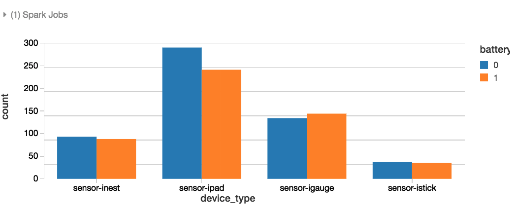
Step 2: Let’s Explore Our Data

display(devicesDF)

Step 3: Visualize our Data

// import some SQL aggregate and windowing function
import org.apache.spark.sql.functions._

val staticCountsDF = devicesDF
    .select("device_type", "battery_level")
    .where ("signal 

Step 4: Stream Processing

Read the stream.

val streamingSignalsCountsDF = streamingDevicesDF
    .select("device_type", "battery_level")
    .where ("signal 

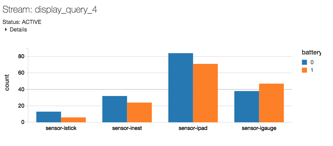
Step 5: Monitor the Stream in Real Time

display(streamingSignalsCountsDF)

Step 6: Model the Data and Optimize the Asset

We have staged some sensor data as a CSV. In the real world, you would read this off the stream as I have shown above. Lets create a temporary table we will use in our analysis.

sqlContext.read.format("csv")
  .option("header", "true")
  .option("delimiter", "\t")
  .option("inferSchema", "true")
  .load("dbfs:/databricks-datasets/power-plant/data/")
  .createOrReplaceTempView("power_plant_sf")

The next step is to prepare the data. Since all of this data is numeric and consistent this is a simple task for us today. We will need to convert the predictor features from columns to Feature Vectors using the org.apache.spark.ml.feature.VectorAssembler. The VectorAssembler will be the first step in building our ML pipeline.

import org.apache.spark.ml.feature.VectorAssembler
val dataset = sqlContext.table("power_plant_sf")
val vectorizer =  new VectorAssembler()
  .setInputCols(Array("AT", "V", "AP", "RH"))
  .setOutputCol("features")

The linear correlation is not as strong between Exhaust Vacuum Speed and Power Output but there is some semblance of a pattern. Now let's model our data to predict what the power output will be given a set of sensor readings.

// First let's hold out 20% of our data for testing and leave 80% for training
var Array(split20, split80) = dataset.randomSplit(Array(0.20, 0.80), 1800009193L)

// Let's cache these datasets for performance
val testSet = split20.cache()
testSet.count()
val trainingSet = split80.cache()
trainingSet.count()

// ***** LINEAR REGRESSION MODEL ****

import org.apache.spark.ml.regression.LinearRegression
import org.apache.spark.ml.regression.LinearRegressionModel
import org.apache.spark.ml.Pipeline

// Let's initialize our linear regression learner
val lr = new LinearRegression()

// Now we set the parameters for the method
lr.setPredictionCol("Predicted_PE")
  .setLabelCol("PE")
  .setMaxIter(100)
  .setRegParam(0.1)
// We will use the new spark.ml pipeline API. If you have worked with scikit-learn this will be very familiar.
val lrPipeline = new Pipeline()
lrPipeline.setStages(Array(vectorizer, lr))
// Let's first train on the entire dataset to see what we get
val lrModel = lrPipeline.fit(trainingSet)

val predictionsAndLabels = lrModel.transform(testSet)

display(predictionsAndLabels.select("AT", "V", "AP", "RH", "PE", "Predicted_PE"))

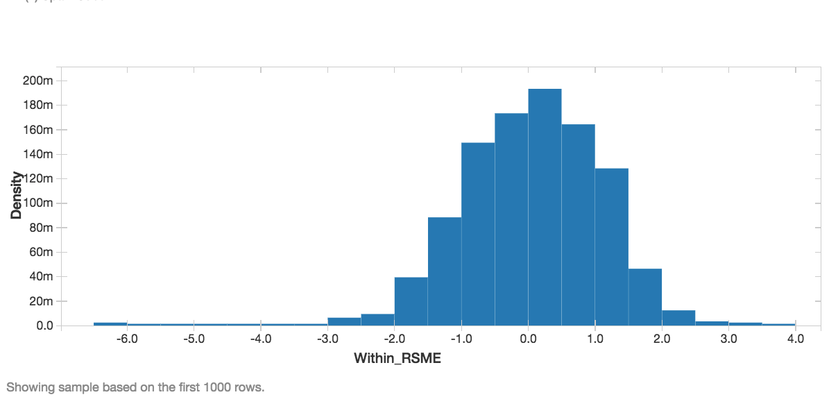
Now that we have real predictions we can use an evaluation metric such as Root Mean Squared Error to validate our regression model. The lower the Root Mean Squared Error, the better our model.

//Now let's compute some evaluation metrics against our test dataset

import org.apache.spark.mllib.evaluation.RegressionMetrics 

val metrics = new RegressionMetrics(predictionsAndLabels.select("Predicted_PE", "PE").rdd.map(r => (r(0).asInstanceOf[Double], r(1).asInstanceOf[Double])))

val rmse = metrics.rootMeanSquaredError
val explainedVariance = metrics.explainedVariance
val r2 = metrics.r2

// First we calculate the residual error and divide it by the RMSE
predictionsAndLabels.selectExpr("PE", "Predicted_PE", "PE - Predicted_PE Residual_Error", s""" (PE - Predicted_PE) / $rmse Within_RSME""").createOrReplaceTempView("Power_Plant_RMSE_Evaluation")

Now we can display the RMSE as a Histogram. Clearly this shows that the RMSE is centered around 0 with the vast majority of the error within 2 RMSEs.

SELECT Within_RSME  from Power_Plant_RMSE_Evaluation

As you can see the Predictions are very close to the real data points. Now we can predict the optimal operating parameters for this plant and apply this model to other plants in real-time.

What’s Next

The example code we used in this blog is available as a Databricks notebook, you can try it with a free trial of Databricks.

This just one of many examples of how Databricks can seamlessly work with other AWS components to deliver advanced solutions. To learn how Databricks helped an energy company analyze IoT data, check out our case study with DNV GL. If you want to get started with Databricks, sign-up for a free trial or contact us.