Simplify Advertising Analytics Click Prediction with Databricks Unified Analytics Platform

Read Rise of the Data Lakehouse to explore why lakehouses are the data architecture of the future with the father of the data warehouse, Bill Inmon.

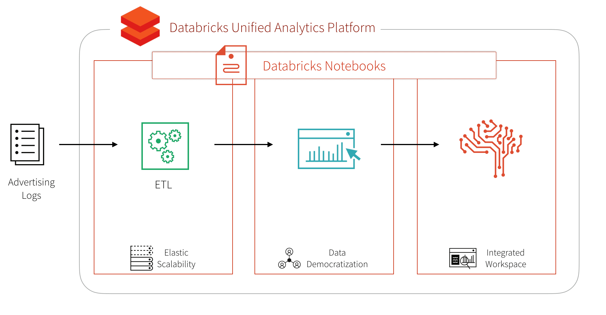
Advertising teams want to analyze their immense stores and varieties of data requiring a scalable, extensible, and elastic platform.  Advanced analytics, including but not limited to classification, clustering, recognition, prediction, and recommendations allow these organizations to gain deeper insights from their data and drive business outcomes. As data of various types grow in volume, Apache Spark provides an API and distributed compute engine to process data easily and in parallel, thereby decreasing time to value.  The Databricks Lakehouse Platform provides an optimized, managed cloud service around Spark, and allows for self-service provisioning of computing resources and a collaborative workspace.

Let's look at a concrete example with the Click-Through Rate Prediction dataset of ad impressions and clicks from the data science website Kaggle.  The goal of this workflow is to create a machine learning model that, given a new ad impression, predicts whether or not there will be a click.

To build our advanced analytics workflow, let’s focus on the three main steps:

• ETL
• Data Exploration, for example, using SQL
• Advanced Analytics / Machine Learning

Building the ETL process for the advertising logs

First, we download the dataset to our blob storage, either AWS S3 or Microsoft Azure Blob storage.  Once we have the data in blob storage, we can read it into Spark.

This creates a Spark DataFrame - an immutable, tabular, distributed data structure on our Spark cluster. The inferred schema can be seen using .printSchema().

To optimize the query performance from DBFS, we can convert the CSV files into Parquet format.  Parquet is a columnar file format that allows for efficient querying of big data with Spark SQL or most MPP query engines.  For more information on how Spark is optimized for Parquet, refer to How Apache Spark performs a fast count using the Parquet metadata.

Explore Advertising Logs with Spark SQL

Now we can create a Spark SQL temporary view called impression on our Parquet files.  To showcase the flexibility of Databricks notebooks, we can specify to use Python (instead of Scala) in another cell within our notebook.

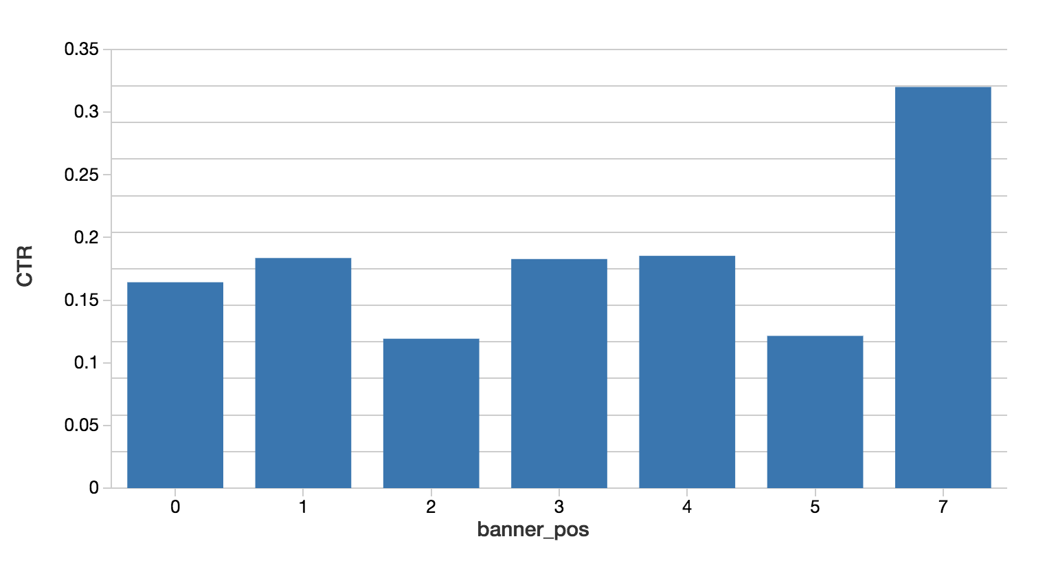
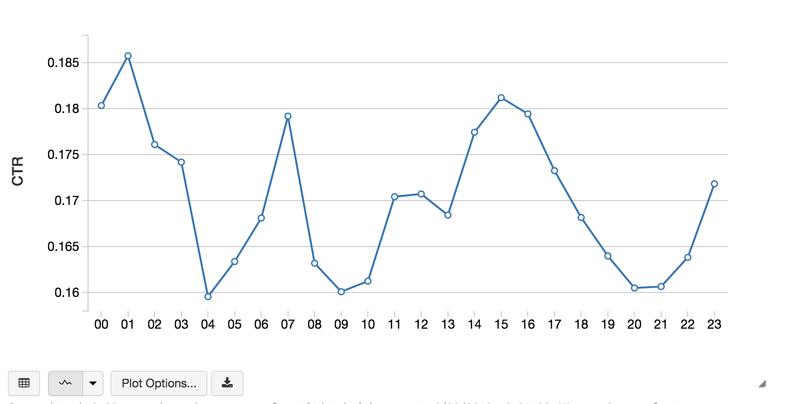
We can now explore our data with the familiar and ubiquitous SQL language. Databricks and Spark support Scala, Python, R, and SQL. The following code snippets calculates the click through rate (CTR) by banner position and hour of day.

Predict the Clicks

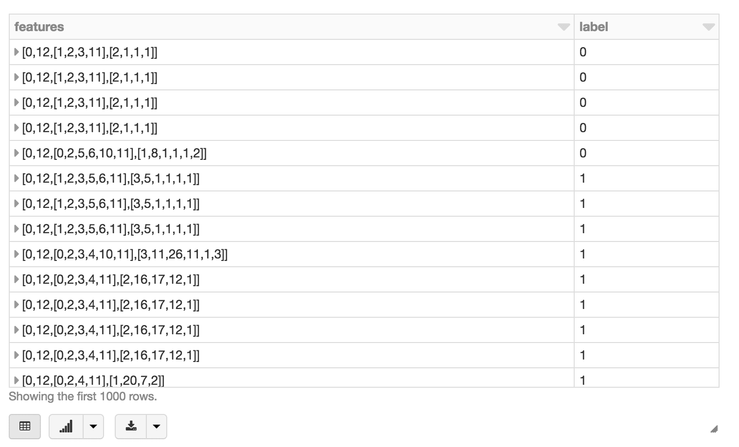
Once we have familiarized ourselves with our data, we can proceed to the machine learning phase, where we convert our data into features for input to a machine learning algorithm and produce a trained model with which we can predict.  Because Spark MLlib algorithms take a column of feature vectors of doubles as input, a typical feature engineering workflow includes:

• Identifying numeric and categorical features
• String indexing
• Assembling them all into a sparse vector

The following code snippet is an example of a feature engineering workflow.

In our use of GBTClassifer, you may have noticed that while we use string indexer but we are not applying One Hot Encoder (OHE). When using StringIndexer, categorical features are kept as k-ary categorical features. A tree node will test if feature X has a value in {subset of categories}. With both StringIndexer + OHE: Your categorical features are turned into a bunch of binary features. A tree node will test if feature X = category a vs. all the other categories (one vs. rest test). When using only StringIndexer, the benefits include: There are fewer features to choose Each node's test is more expressive than with binary 1-vs-rest features Therefore, for because for tree based methods, it is preferable to not use OHE as it is a less expressive test and it takes up more space. But for non-tree-based algorithms such as like linear regression, you must use OHE or else the model will impose a false and misleading ordering on categories. Thanks to Brooke Wenig and Joseph Bradley for contributing to this post!

With our workflow created, we can create our ML pipeline.

Using display(featurizedImpressions.select('features', 'label')), we can visualize our featurized dataset.

Next, we will split our featurized dataset into training and test datasets via .randomSplit().

Next, we will train, predict, and evaluate our model using the GBTClassifier.  As a side note, a good primer on solving binary classification problems with Spark MLlib is Susan Li’s Machine Learning with PySpark and MLlib — Solving a Binary Classification Problem.

With our predictions, we can evaluate the model according to some evaluation metric, for example, area under the ROC curve, and view features by importance.  We can also see the AUC value which in this case is 0.7112027059.

Summary

We demonstrated how you can simplify your advertising analytics - including click prediction - using the Databricks Unified Analytics Platform (UAP). With Databricks UAP, we were quickly able to execute our three components for click prediction: ETL, data exploration, and machine learning.  We’ve illustrated how you can run our advanced analytics workflow of ETL, analysis, and machine learning pipelines all within a few Databricks notebook.

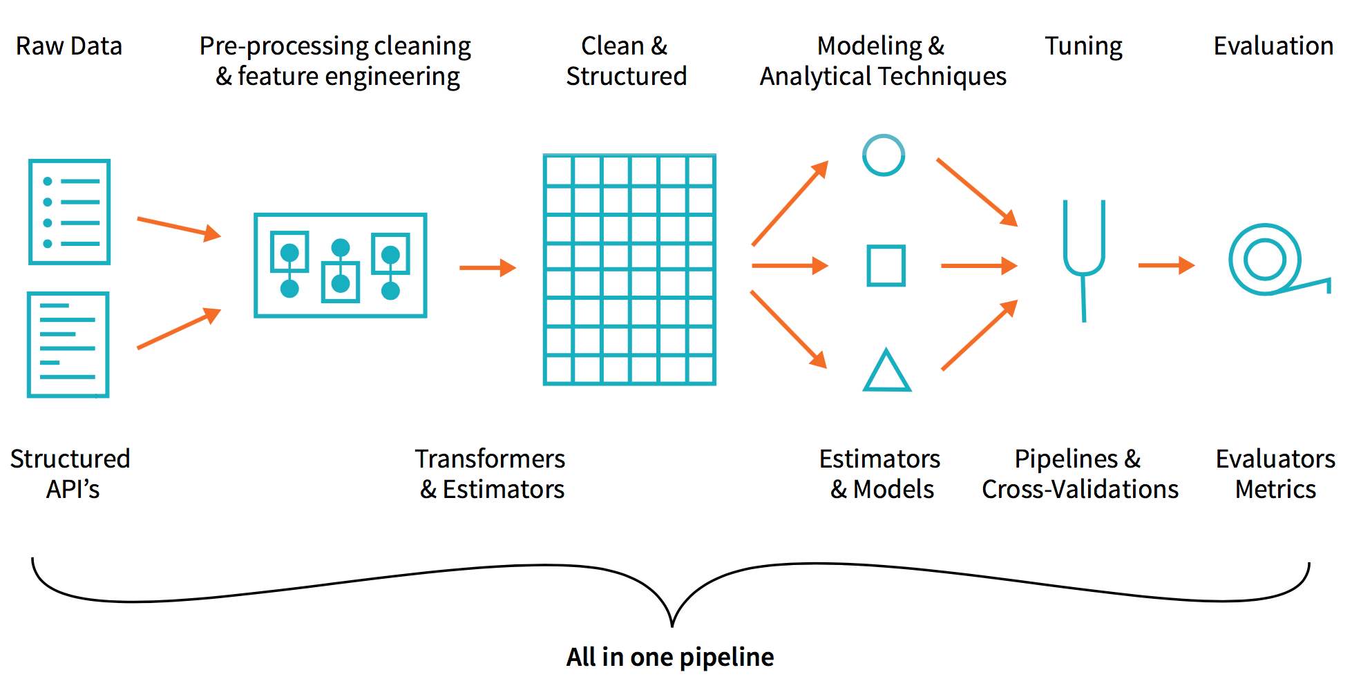
By removing the data engineering complexities commonly associated with such data pipelines with the Databricks Unified Analytics Platform, this allows different sets of users i.e. data engineers, data analysts, and data scientists to easily work together.