How the Minnesota Twins Scaled Pitch Scenario Analysis to Measure Player Performance - Part 1

Statistical Analysis in the Game of Baseball 

A single pitch in Major League Baseball (MLB) generates tens of megabytes of data, from pitch movement to ball rotation to hitter  behavior to the movement of each individual baseball player in response to a hit. How do you derive actionable insights from all this data over the course of a game and season? Learn how the Baseball Operations Group within the 2019 AL Central Division Champion Minnesota Twins is using Databricks to take reams of sensor data, run thousands or tens of thousands of simulations on each pitch, and then quickly generate actionable insights to analyze and improve player performance, scout the competition, and better evaluate talent. Additionally, learn how they are planning to shorten the analysis cycle even further to get these insights to the coaches in order to optimize in-game strategy based on real-time action.

In part 1, we walk through the challenges the Twins’ front office was facing in running thousands of simulations on their pitch data to improve their player evaluation model. We evaluate the tradeoffs around different methodologies for modeling and inferring pitch outcomes in R, and why we chose to proceed with user defined function with R in Spark.

In part 2, we take a deeper dive into user defined functions with R in Spark. We will learn how to optimize performance to enable scale by managing the behavior of R inside the UDF as well as the behavior of Spark as it orchestrates execution.

Background

There are several discrete baseball statistics that can be used to evaluate a baseball player’s’ performance such as batting average or runs batted in, but the sabermetric baseball community developed Wins Above Replacement (WAR) to estimate a players’ total contribution to the team’s success in a way to make it easier to compare players. From FanGraphs.com:

You should always use more than one metric at a time when evaluating players, but WAR is all-inclusive and provides a useful reference point for comparing players. WAR offers an estimate to answer the question, “If this player got injured and their team had to replace them with a freely available minor leaguer or a AAAA player from their bench, how much value would the team be losing?” This value is expressed in a wins format, so we could say that Player X is worth +6.3 wins to their team while Player Y is only worth +3.5 wins, which means it is highly likely that Player X has been more valuable than Player Y.

Historically, comparing players’ WAR over the course of hundreds or thousands of pitches was the best way to gauge relative value. The Minnesota Twins had data on over 15 million pitches that included not just final outcome (ball, strike, base hit, etc), but also deeper data like ball speed and rotation, exit velocity, player positioning, fielding independent pitching (FIP), and so on. However, any single pitch can have several variables, like batter-pitcher pairing or weather, that affect the play’s expected run value (e.g., the breeze picks up and what could have been a homerun instead becomes a foul ball). But how do you correct for those variables in order to derive a more accurate prediction of future performance?

Based on the law of large numbers, industries like Financial Services run Monte Carlo simulations on historical data to increase the accuracy of their probabilistic models. Similarly, a 100-fold increase in scenarios (think of each pitch as a scenario) leads to a 10-fold more accurate WAR estimate. To increase the accuracy of their expected run value, the Twins looked for a solution that could generate up to 20,000 simulations on each of the pitches in their database, or up to 300 billion scenarios total (15 million pitches x 20,000 simulations per pitch in max scenario = 300 billion total scenarios). Running this analysis  on-prem with Base R on a single node, they realized it would take almost four years to compute the historical data (~8 seconds to run 20k simulations per pitch x 15 million pitches / 3.15x107 seconds per year). If they were going to eventually use run value/WAR estimates to optimize in-game decisions, where each game could generate over 40,000 scenarios to score, they needed:

1. A way to quickly spin up massive amounts of compute power for short periods of time and
2. A living model where they could continuously add new baseball data to improve the accuracy of their forecasts and generate actionable insights in near real time.

The Twins turned to Databricks and Microsoft Azure, given our experience with massive data sets that include both structured and unstructured data. With the near limitless on-demand compute available in the cloud, the Twins no longer had to worry about provisioning hardware for a one-time spike in use around analyzing the historical data. Where previously running 40,000 daily simulations would have taken 44 minutes, with Databricks on Azure they unlocked the capability for real-time scoring as data gets generated.

Scaling Pitch Simulation Outcomes by 100X

Modeling and Inferring Pitch Outcomes in R

To model the outcome of a given pitch, the data science team settled on a training dataset consisting of 15 million rows with pitch location coordinates as well as season and game features like pitcher-batter handedness, inning, and so on.  In order to capture the non-linear properties of pitch outcomes in their models, the team turned to the vast repository of open source packages available in the R ecosystem.

Ultimately an R package was chosen that was particularly useful for its flexibility and interpretability when modeling non-linear distributions.  Data scientists could fit a complex model on historical data and still understand the precise effect each predictor has on the pitch outcome.   Since the models would be used to help evaluate player performance and team composition, interpretability of the model was an important consideration for coaches and the business.

Having modeled various pitch outcomes, the team then used R to simulate the joint probability distribution of x-y coordinates for each pitch in the dataset.  This effectively generated additional records that could be scored with their trained models.  Inferring the expected pitch outcome for each simulated pitch sketches an image of expected player performance.   The greater the number of simulations the sharper that image becomes.

A plan was made to generate 20,000 simulations for each one of the 15 million rows in the historical dataset.  This would yield a final dataset of 300 billion simulated pitches ready for inference with their non-linear models, and provide the organization with the data to evaluate their players more accurately.

The problem with this approach was that by nature R operates in a single threaded, single node execution environment.  Even when leveraging the multi-threading packages available in open source and a CPU heavy VM in the cloud, the team estimated that it would take months for the code to complete, if it completed at all.  The question became one of scale:  How can the simulation and inference logic scale to 300 billion rows and complete the job in a reasonable time frame?  The answer lay in the Databricks Unified Analytics Platform powered by Apache Spark.

Scaling R with Spark 

The first step in scaling this simulation pipeline was to refactor the feature engineering code to work with one of the two packages available in R for Spark - SparkR or sparklyr.  Luckily, they had written their logic using the popular data manipulation package dplyr, which is tightly integrated with sparklyr. This integration enables the use of dplyr functions on the tbl_spark objects created when reading data with sparklyr.  In this instance we only had to convert a few ifelse() statements to dplyr::mutate(case_when(...)), and then their feature engineering code would scale from a single node process to a massively parallel workload with Spark!  In fact, about only 10% of the existing dplyr code needed to be refactored to work with Spark.  We were now able to generate billions of rows for inference in a matter of minutes.

How does this dplyr magic work?  To understand this we need to first understand how the R to Spark interface is structured:

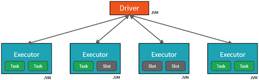
Most of the functions in the Spark + R packages are wrappers around native Spark classes - your R code gets translated into Scala, and those commands are sent to the JVM on the driver where tasks are then assigned to each worker.  In a similar vein, dplyr verbs are translated into SQL expressions that are then evaluated by Spark through SparkSQL.  As a result one generally should see the same performance in Spark + R packages that you would expect in Scala.

Distributed Inference with R Packages 

With the feature engineering pipeline running in Spark, our attention turned towards scaling model inference. We considered three distinct approaches:

• Retrain the non-linear models in Spark
• Extract the model coefficients from R and score in Spark
• Embed the R models in a user defined function and parallelize execution with Spark

Let’s briefly examine the feasibility and tradeoffs associated with each of these approaches.

Retrain the Non-linear Models in Spark

The first approach was to see if an implementation of the modeling technique from R existed in Spark’s machine learning library (SparkML).  In general, if your model type is available in SparkML it is best to choose that for performance, stability, and simpler debugging. This can require refactoring code somewhat if you are coming from R or Python, but the scalability gains can easily make it worth it.

Unfortunately the modeling approach chosen by the team is not available in SparkML. There has been some work done in academia, but since it involved introducing modifications to the codebase in Spark we decided to deprioritize this approach in favor of alternatives. The amount of work required to refactor and maintain this code made it prohibitive to use as a first approach.

Extracting Model Coefficients 

If we couldn’t retrain in Spark, perhaps we could use the learned coefficients from R models and apply them to a Spark DataFrame?  The idea here is that inference can be performed by multiplying an input DataFrame of features by a smaller DataFrame of coefficients to arrive at predicted values. Again, the tradeoff would be some refactoring code to orchestrate coefficient extraction from R to Spark in order to gain massive scalability and performance.

For this approach to work with this type of non-linear model, we would need to extract a matrix of linear predictors along with the model coefficients.  Due to the nature of the R package being used, this matrix cannot be generated without passing new data through the R model object itself.  Generating a matrix of linear predictors from 300 billion rows is not feasible in R, and so the second approach was abandoned.

Parallelizing R Execution with User Defined Functions in Spark

Given the lack of native support for this particular non-linear modeling approach in Spark and the futility of generating a 300 billion row matrix in R, we turned to User Defined Functions (UDFs) in SparkR and sparklyr.

In order to understand UDFs, we need to take a step back and reconsider the Spark and R architecture shown above.

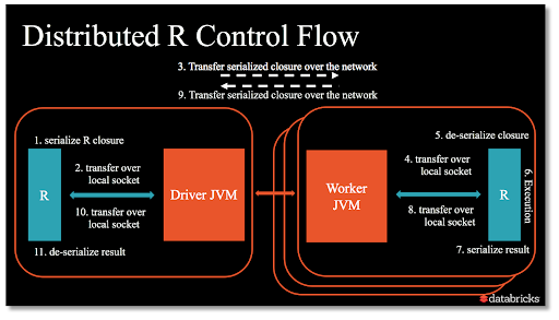
With UDFs, the pattern changes somewhat from before.  UDFs create an R process on each worker, enabling the user to execute arbitrary R code in parallel across the cluster.  These functions can be applied to a partition or group of a Spark DataFrame, and will return the results back as a Spark DataFrame. Another way to think of this is that UDFs provide access to the R console on each worker, with the ability to apply an R function to data there and return the results back to Spark.

To perform inference on billions of rows with a model type not available in SparkML, we loaded the simulation data into a Spark DataFrame and applied an R function to each partition using SparkR::dapply. The high-level structure of our function was as follows.

results <- dapply(features,
	# x is a partition of data
    function(x) {

    # load model object
    model <- readRDS(“/dbfs/pitch_outcome_model.rds”)

    # infer pitch outcomes 
    x$predictions <- predict(model, data = x)

    # return result
    x
    },  schema = schema)

Let’s break this function down further.  For each partition of data in the features Spark DataFrame we apply an R function to:

• Load an R model into memory from the Databricks File System (DBFS)
• Make predictions in R
• Return the resulting dataframe back to Spark
• Specify output schema for the results Spark DataFrame

DBFS is a path mounted on each node in the cluster that points to cloud storage, and is accessible from R.  This makes it easy to load models on the workers themselves instead of broadcasting them as variables across the network with Spark.  Ultimately, this third approach proved fruitful and allowed the team to scale their models trained in R for distributed inference on billions of rows with Spark.

Conclusion

In this post we reviewed a number of different approaches for scaling simulation and player valuation pipelines written in R for the Minnesota Twins MLB team.  We walked through the reasoning for choosing various approaches, the tradeoffs, and the architectural differences between core SparkR/sparklyr functions and user defined functions.

From feature engineering to model training, coefficient extraction, and finally user defined functions it is clear that plenty of options exist to extend the power of the R ecosystem to big data.

In the next post we will take a deeper dive into user defined functions with R in Spark.  We will learn how to optimize performance by managing the behavior of R inside the UDF as well as the behavior of Spark as it orchestrates execution.

Check out part 2 of the Minnesota Twins story: Optimizing UDF with Apache Spark and R