Modernizing Risk Management Part 2: Aggregations, Backtesting at Scale and Introducing Alternative Data

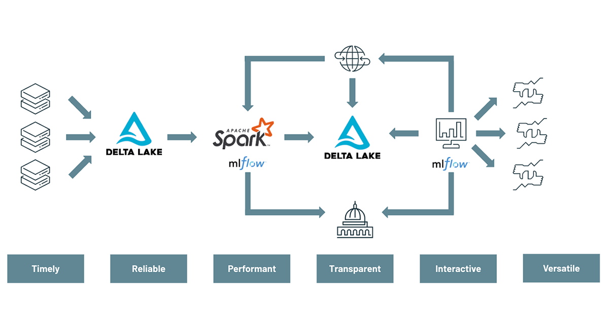
Understanding and mitigating risk is at the forefront of any financial services institution. However, as previously discussed in the first blog of this two-part series, banks today are still struggling to keep up with the emerging risks and threats facing their business. Plagued by the limitations of  on-premises infrastructure and legacy technologies, banks until recently have not had the tools to effectively build a modern risk management practice. Luckily, a better alternative exists today based on open-source technologies powered by cloud-native infrastructure. This Modern Risk Management framework  enables intraday views, aggregations on demand and an ability to future proof/scale risk management. In this two-part blog series, we demonstrate how to modernize traditional value-at-risk calculation through the use of Delta Lake, Apache Spark^TM and MLflow in order to enable a more agile and forward looking approach to  risk management.

The first demo addressed the technical challenges related to modernizing risk management practices with data and advanced analytics, covering the concepts of risk modelling and Monte Carlo simulations using MLflow and Apache Spark^TM. This article focuses on the risk analyst persona and their requirements to efficiently slice and dice risks simulations (on demand) in order to better understand portfolio risks as new threats emerge, in real time. We will cover the following topics:

• Using Delta Lake and SQL for aggregating value-at-risk on demand
• Using Apache Spark^TM and MLflow to backtest models and report breaches to regulators
• Exploring the use of alternative data to better assess your risk exposure

Slicing and dicing value-at-risk with Delta Lake

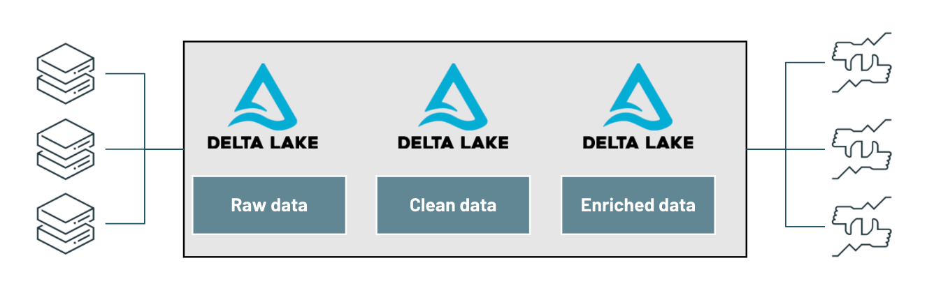
In part one of this two-part blog series, we unveiled what a modern risk management platform looks like and the need for FSIs to shift the lense in which data is viewed: not as a cost, but as an asset. We demonstrated the versatile nature of data, and how storing Monte Carlo data in its most granular form would enable multiple use-cases along with providing analysts with the flexibility to run ad-hoc analysis, contributing to a more robust and agile view of the risks banks are facing.

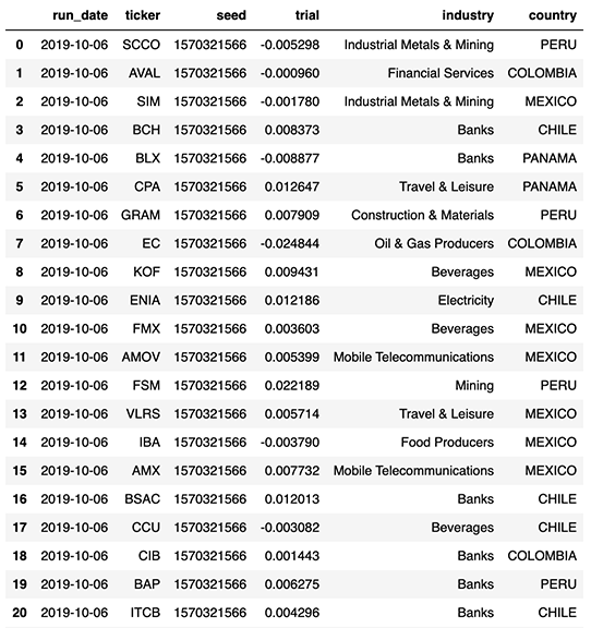
In this blog and demo, we uncover the risk of various investments in a Latin America equity portfolio composed of 40 instruments across multiple industries. For that purpose, we leverage the vast amount of data we were able to generate through Monte Carlo simulations (40 instruments x 50,000 simulations x 52 weeks = 100 million records), partitioned by day and enriched with our portfolio taxonomy as follows.

Value-at-risk

Value-at-risk is the process of simulating random walks that cover possible outcomes as well as worst case (n) scenarios. A 95% value-at-risk for a period of (t) days is the best case scenario out of the worst 5% trials.

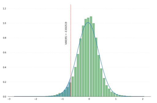
As our trials were partitioned by day, analysts can easily access a day’s worth of simulations data and group individual returns by a trial Id (i.e. the seed used to generate financial market conditions) in order to access the daily distribution of our investment returns and its respective value-at-risk.  Our first approach is to use Spark SQL to aggregate our simulated returns for a given day (50,000 records) and use in-memory python to compute the 5% quantile through a simple numpy operation.

returns = spark \
    .read \
    .table(monte_carlo_table) \
    .filter(F.col('run_date') == '2020-01-01') \
    .groupBy('seed') \
    .agg(F.sum('trial').alias('return')) \
    .select('return') \
    .toPandas()['return']

value_at_risk = np.quantile(returns, 5 / 100)

Provided an initial $10,000 investment across all our Latin American equity instruments, the 95% value-at-risk - at that specific point in time - would have been $3,000. This is how much our business would be ready to lose (at least) in the worst 5% of all the possible events.

The downside of this approach is that we first need to collect all daily trials in memory in order to compute the 5% quantile. While this process can be performed easily when using 1 day worth of data, it quickly becomes a bottleneck when aggregating value-at-risk over a longer period of time.

A pragmatic and scalable approach to problem solving

Extracting percentile from a large dataset is a known challenge for any distributed computing environment. A common (albeit inefficient) practice is to 1) sort all of your data and 2) cherry pick a specific row using takeOrdered or to find an approximation through the approxQuantile method. Our challenge is slightly different since our data does not constitute a single dataset but spans across multiple days, industries and countries, where each bucket may be too big to be efficiently collected and processed in memory.

In practice, we leverage the nature of value-at-risk and only focus on the worst n events (n small). Given 50,000 simulations for each instrument and a 99% VaR, we are interested in finding the best of the worst 500 experiments only. For that purpose, we create a user defined aggregate function (UDAF) that only returns the best of the worst n events. This approach will drastically reduce the memory footprint and network constraints that may arise when computing large scale VaR aggregation.

class ValueAtRisk(n: Int) extends UserDefinedAggregateFunction {

    // These are the input fields for your aggregate function.
    override def inputSchema: org.apache.spark.sql.types.StructType = {
        StructType(StructField("value", DoubleType) :: Nil)
    }
    
    // These are the internal fields you keep for computing your aggregate.
    override def bufferSchema: StructType = StructType(
        Array(
            StructField("worst", ArrayType(DoubleType))
        )
    )
    
    // This is the output type of your aggregation function.
    override def dataType: DataType = DoubleType
    
    // The order we process dataframe does not matter
    // the worst will always be the worst
    override def deterministic: Boolean = true
    
    // This is the initial value for your buffer schema.
    override def initialize(buffer: MutableAggregationBuffer): Unit = {
        buffer(0) = Seq.empty[Double]
    }
    
    // This is how to update your buffer schema given an input.
    override def update(buffer: MutableAggregationBuffer, input: Row): Unit = {
        buffer(0) = buffer.getAs[Seq[Double]](0) :+ input.getAs[Double](0)
    }
    
    // This is how to merge two objects with the bufferSchema type.
    // We only keep worst N events
    override def merge(buffer: MutableAggregationBuffer, row: Row): Unit = {
        buffer(0) = (
            buffer.getAs[Seq[Double]](0) ++ row.getAs[Seq[Double]](0)
        ).sorted.take(n)
    }
    
    // This is where you output the final value
    // Our value at risk is best of the worst n overall
    override def evaluate(buffer: Row): Any = {
        return buffer.getAs[Seq[Double]](0).sorted.last
    }
    
}

// 95% value at risk is the best of the worst N events 
val n = (100 - 95) * numSimulations / 100

// Register UADFs
spark.udf.register("VALUE_AT_RISK", new ValueAtRisk(n))

By registering our UADF through spark.udf.register method, we expose that functionality to all of our users, democratizing risk analysis to everyone without an advanced knowledge of scala / python / spark. One simply has to group by trial Id (i.e. seed) in order to apply the above and extract the relevant value-at-risk using plain old SQL capabilities across all their data.

SELECT 
    t.run_date AS day, 
    VALUE_AT_RISK(t.return) AS value_at_risk
FROM 
    (
    SELECT 
        m.run_date, 
        m.seed, 
        sum(m.trial) AS return
    FROM
        monte_carlo m
    GROUP BY
        m.run_date, 
        m.seed 
    ) t
GROUP BY 
    t.run_date
ORDER BY t.run_date ASC

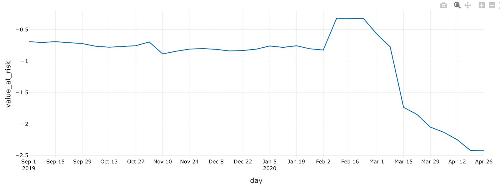
We can easily uncover the effect of COVID-19 on our market risk calculation. A 90-day period of economic volatility resulted in a much lower value-at-risk and therefore a much higher risk exposure overall since early March 2020.

Holistic view of our risk exposure

In most cases, understanding overall value-at-risk is not enough. Analysts need to understand the risk exposure to different books, asset classes, different industries or different countries of operations. In addition to Delta Lake capabilities such as time travel and ACID transactions discussed earlier, Delta Lake and Apache Spark^TM have been highly optimised on Databricks runtime to provide fast aggregations at read. High performance can be achieved using our native partitioning logic (by date) alongside a z-order indexing applied to both country and industry. This additional indexing will be fully exploited when selecting a specific slice of your data at a country or industry level, drastically reducing the amount of data that needs to be read prior to your VaR aggregation.

OPTIMIZE monte_carlo ZORDER BY (country, industry)

We can easily adapt the above SQL code by using country and industry as our grouping parameter for VALUE_AT_RISK method in order to have a more granular and descriptive view of our risk exposure. The resulting data set can be visualised “as-is” using Databricks notebook and can be further refined to understand the exact contribution each of these countries have to our overall value-at-risk.

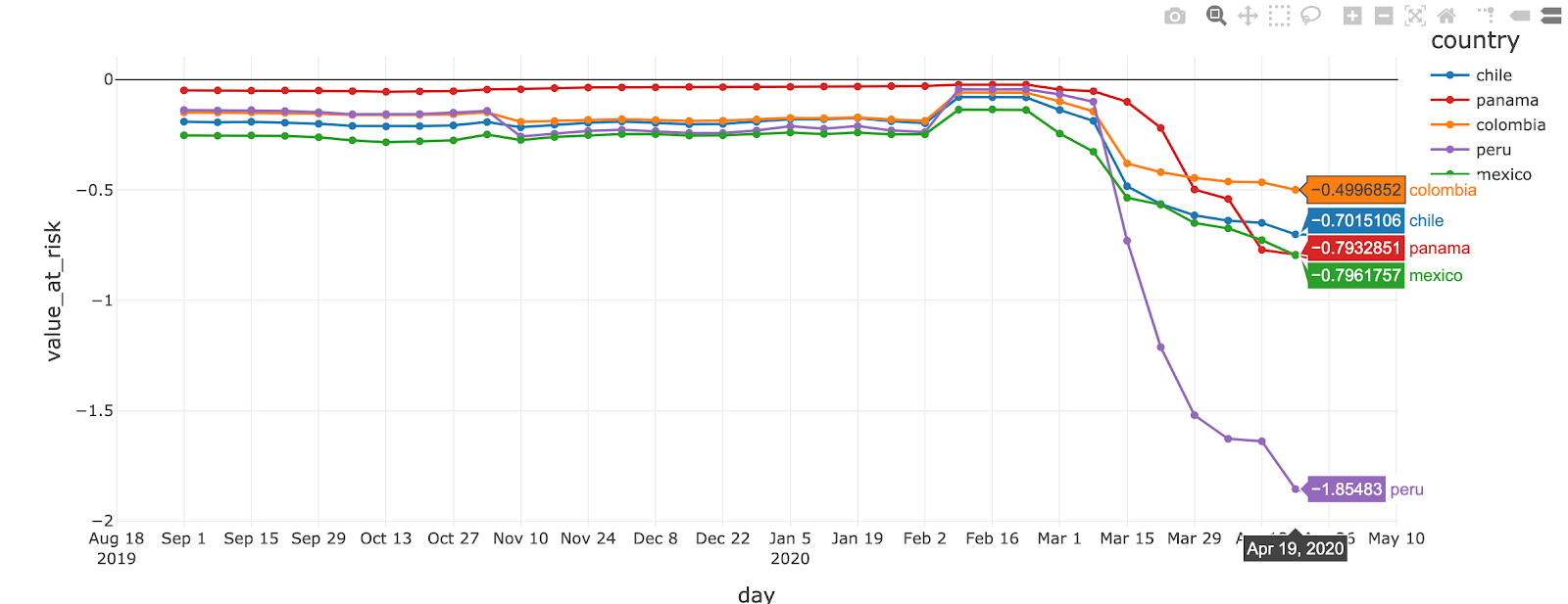
In this example, Peru seems to have the biggest contribution to our overall risk exposure. Looking at the same SQL code at an industry level in Peru, we can investigate the contribution of the risk across industries.

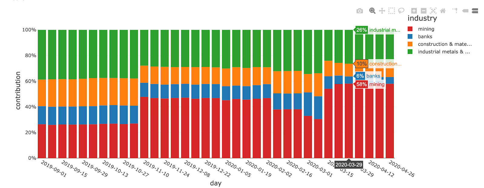
With a contribution close to 60% in March 2020, the main risk exposure in Peru seems to be related to the mining industry. An increasingly severe lockdown in response to the COVID virus has been impacting mining projects in Peru, centre for copper, gold and silver production (source).

Stretching the scope of this article, we may wonder if we could have identified this trend earlier using alternative data and specifically the global database of events, locations and tone (GDELT). We report in below graph the media coverage for the mining industry in Peru, color coding positive and negative trends through a simple moving average.

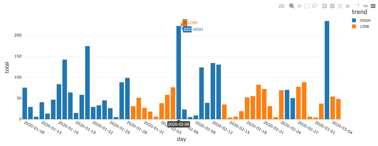
This clearly exhibits a positive trend in early February, i.e. 15 days prior to the observed stock volatility, which could have been an early indication of mounting risks. This analysis stresses the importance of modernizing value-at-risk calculations, augmenting historical data with external factors derived from alternative data.

Model backtesting

In response to the 2008 financial crisis, an additional set of measures were developed by the Basel committee on banking supervision. The 1 day VaR 99 results are to be compared against daily P&Ls. Backtests are to be performed quarterly using the most recent 250 days of data. Based on the number of exceedances experienced during that period, the VaR measure is categorized as falling into one of three colored zones.

AS-OF value-at-risk

Given the aggregated function we defined earlier, we can extract daily value-at-risk across our entire investment portfolio. As our aggregated value-at-risk dataset is small (contains 2 years of history, i.e. 365 x 2 data points), our strategy is to collect daily VaR and broadcast it to our larger set in order to avoid unnecessary shuffles. More details on AS-OF functionalities can be found in an earlier blog post Democratizing Financial Time Series Analysis.

case class VarHistory(time: Long, valueAtRisk: String)

val historicalVars = sql(s"""
    SELECT t.run_date, VALUE_AT_RISK(t.return) AS valueAtRisk
    FROM 
        (
        SELECT m.run_date, m.seed, sum(m.trial) AS return
        FROM monte-carlo m
        GROUP BY m.run_date, m.seed
        ) t
    GROUP BY 
        t.run_date
    """
    )
    .withColumn("time", convertDate(col("run_date")))
    .orderBy(asc("time"))
    .select("time", "valueAtRisk")
    .as[VarHistory]
    .collect()
    .sortBy(_.time)
    .reverse

val historicalVarsB = spark.sparkContext.broadcast(historicalVars)

We retrieve the closest value-at-risk to our actual returns via a simple user defined function and perform a 250-day sliding window to extract continuous daily breaches.

val asOfVar = udf((s: java.sql.Date) => {
    val historicalVars = historicalVarsB.value
    if(s.getTime  s.getTime)
            .headOption.map(_.valueAtRisk) 
    }
})

val windowSpec = Window.orderBy("time").rangeBetween(-3600 * 24 * 250, 0)
val countBreaches = udf((asOfVar: Double, returns: Seq[Double]) => {
    returns.count(_ 

We can observe a consecutive series of 17 breaches from February onwards that would need to be reported to regulations according to the Basel III framework. The same can be reported onto a graph, over time.