Analyzing Algorand Blockchain Data With Databricks Delta (Part 2)
by Anindita Mahapatra and Eric Gieseke
Get an early preview of O'Reilly's new ebook for the step-by-step guidance you need to start using Delta Lake.
This post was written in collaboration betweeen Eric Gieseke, principal software engineer at Algorand, and Anindita Mahapatra, solutions architect, Databricks.
Algorand is a public, decentralized blockchain system that uses a proof of stake consensus protocol. It is fast and energy efficient, with a transaction commit time under five seconds and a throughput of one thousand transactions per second. Blockchain is a disruptive technology that will transform many industries including Fintech. Algorand, being a public blockchain, generates large amounts of transaction data and this provides interesting opportunities for data analysis.
Databricks provides a Unified Data Analytics Platform for massive-scale data engineering and collaborative data science on multi-cloud infrastructure. This blog post will demonstrate how Delta Lake facilitates real-time data ingestion, transformation, and SQL Analytics visualization of the blockchain data to provide valuable business insights. SQL is a natural choice for business analysts who benefit from SQL Analytics’ out-of-box visualization capabilities. Graphs are also a powerful visualization tool for blockchain transaction data. This article will show how Apache Spark™ GraphFrame and graph visualization libraries can help analysts identify significant patterns.
This article is the second part of a two part blog. In part one, we demonstrated the analysis of operational telemetry data. In part two, we will show how to use Databricks to analyze the transactional aspects of the Algorand blockchain. A robust ecosystem of accounts, transactions and digital assets is essential for the health of the blockchain. Assets are digital tokens that represent reward tokens, cryptocurrencies, supply chain assets, etc. The Algo digital currency price reflects the intrinsic value of the underlying blockchain. Healthy transaction volume indicates user engagement.
Data processing includes ingestion, transformation and visualization of Algorand transaction data. The insights derived from the resulting analysis will help in determining the health of the ecosystem. For example:
- Which assets are driving transaction volume? What is the daily trend of transaction volume? How does it vary over time? Are there certain times of the day that transaction volumes peak?
- Which applications or business models are driving growth in the number of accounts or transactions?
- What are the distribution of asset types and transaction types? Which assets are most widely used, and which assets are trending up or down?
- What is the latest block? How long did it take to create, and what are the transactions that it contains?
- Which are the most active accounts, and how does their activity vary over time?
- What is the relationship between accounts? Is it possible to detect illicit activity?
- How does the Algo price vary with the transaction volume over time? Can fluctuations in price or volume be predicted?
Algorand network
The Algorand Blockchain network is composed of nodes and relays hosted on servers connected via the internet. The nodes provide the compute and storage needed to host the immutable blocks. The blocks hold the individual transactions committed on the blockchain, and each block links to the preceding block in the chain.
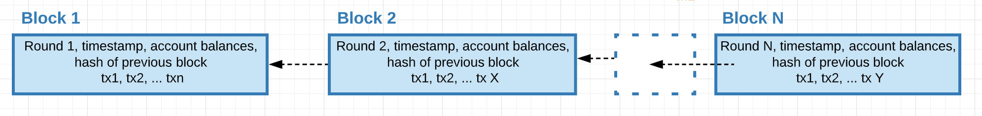
Figure 1: Each block is connected to the prior block to form the blockchain
Algorand data
| Data Type | What | Why | Where |
| Node Telemetry
(JSON data from ElasticSearch API) |
Peer connection data that describes the network topology of nodes and relays | It gives a real-time view of where the nodes & relays are and how they are connected and are communicating, and the network load. | The nodes periodically transmit this information to a configured ElasticSearch endpoint. |
| Block, Transaction, Account Data
(JSON/CSV data from S3) |
Transaction data committed into blocks chained sequentially and individual account balances | This data gives visibility into usage of the blockchain network and people (accounts) transacting. Each account is an established identity, and each tx/block has a unique identifier. | The Algorand blockchain generates block, account, and transaction data. The Algorand Indexer aggregates the data, which is accessible via a REST API. |
Block, transaction and account data
The Algorand blockchain uses an efficient and high-performance consensus protocol based on proof of stake, which enables a throughput of 1,000 transactions per second.
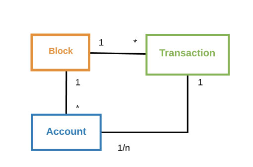 |
Transactions transfer value between Accounts.
Blocks aggregate Transactions that are committed to the blockchain. A new Block is created in less than 5 seconds and is linked to the previous Block to form the blockchain. |
Figure 2: Entity Relation
Analytics workflow
The following diagram describes the data flow. Originating from the Algorand Nodes, blocks are aggregated by the Algorand Indexer into a Postgres database. A Databricks job uses the Algorand Python SDK to retrieve blocks from the Indexer as JSON documents and stores them in an S3 bucket. Using the Databricks Autoloader, the JSON documents are auto-ingested from S3 into Delta Tables as they arrive. Additional processing converts the block records to transaction records in a silver table. Then, from the transaction records, aggregates are produced in the gold table. Both the silver and gold tables support visualization and analytics.
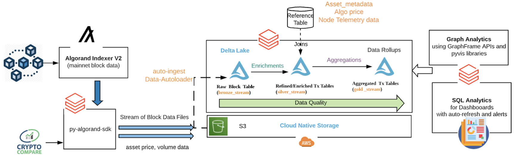
Figure 3: Analytic Workflow
As the blockchain creates new blocks, our streaming pipeline automatically updates the Delta tables with the latest transaction and account data. The processing steps follow:
- Data ingestion
-
- Fetch data as JSON files using the
- into an S3 bucket:
-
- Block data containing transactions (sender, payer, amount, fee, time, type, asset type)
- Account balances (account, asset, balance)
- Asset data (asset id, asset name, unit name)
- Algo Trading details using the CryptoCompare API (time, price, volume). This trading data will augment the transaction data to correlate the Algo price with the transaction activity.
- Auto Data Loader
-
- The
- adds new block data into the 'bronze' Delta table as a real-time streaming job.
- Data refinement
-
- A second streaming job reads the block data from the bronze table, flattens the blocks into individual transactions, and stores the resulting transactions into the 'silver' Delta table.
- Additional transformations include:
-
- Compute statistics for each block, e.g., block time and number of transactions
- A User-Defined Function (UDF) extracts the note field from each transaction, decodes, and removes non-ASCII characters.
- Compute word counts from the processed note field to determine trending words.
- InStream aggregation
- Compute in-stream aggregation statistics on transaction data from the silver table and persist into the 'gold’ Delta table.
-
- Compute count, sum, average, min, max of transaction amounts grouped hourly over each asset type to study trends over time
- Analysis
- Perform Data Analysis and Visualization using the silver and gold tables.
-
- Using GraphFrames & pyvis
- Create vertices and edges from the transaction data to form a directed graph representing accounts as vertices and transactions as edges.
- Using Graph APIs, analyze the data for top users and their incoming/outgoing transactions.
- Visualize the resulting graph using pyvis.
- Using SQL Analytics
- Use SQL queries to analyze data in the Delta Lake and build parameterized Redash dashboards with alerting webhooks.
- Using GraphFrames & pyvis
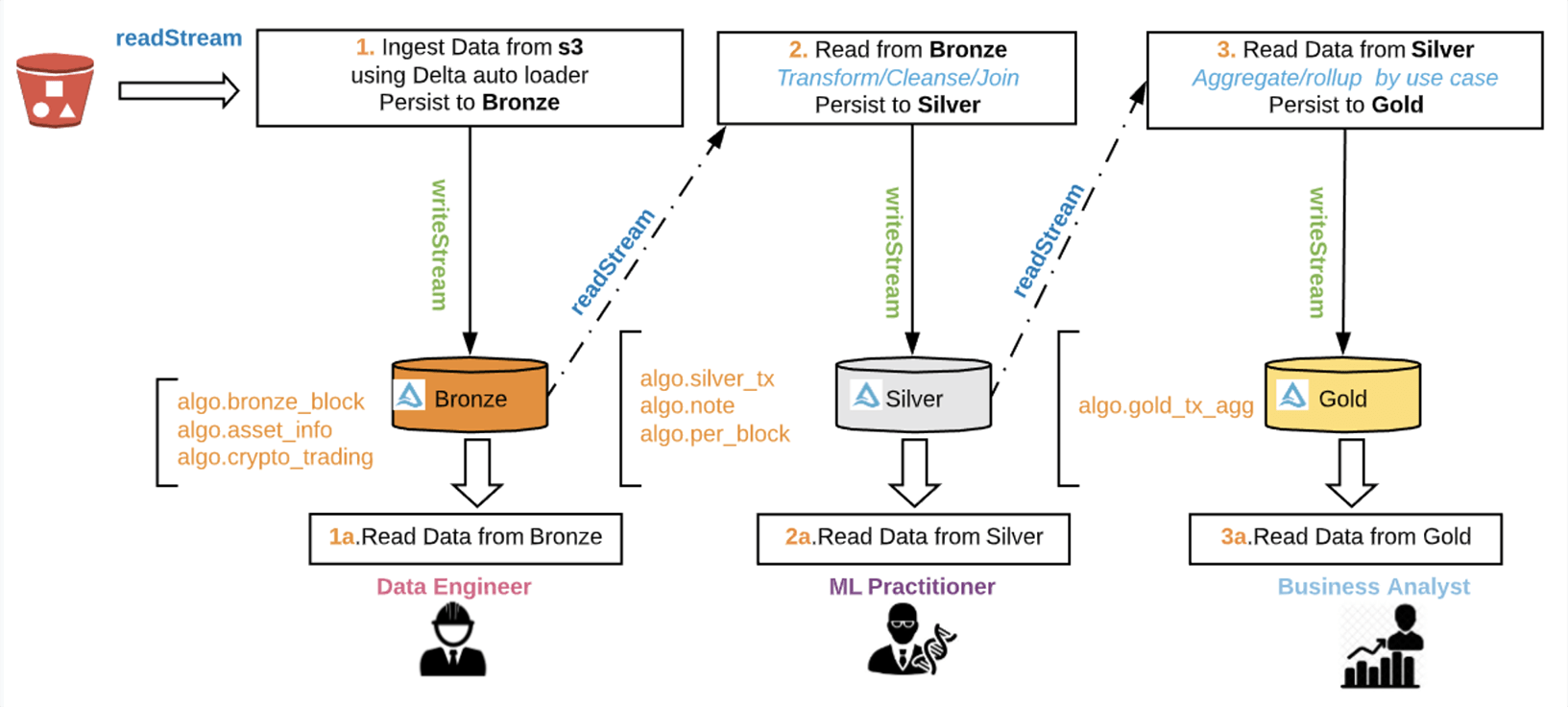
Figure 4: Multihop Data Flow
Step 1: Data ingestion into S3
This notebook is run as a Periodic Job to retrieve new algorand blocks as JSON files from Algorand Indexer V2 into the S3 bucket location. It also retrieves and refreshes the asset information.
- With%pip, install the notebook-scoped library.
- Databricks Secretssecurely stores credentials and sensitive information.
- For the initial bulk load of historical block data, a Spark UDFutilizes the distributed computing of the Spark worker nodes.
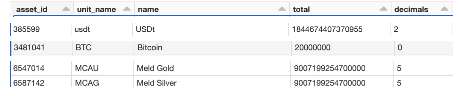
- A transaction can be associated with any asset type–the asset information has details on each asset created on the blockchain, including the ID, unit, name and decimals. The decimals specify the number of zeros following the decimal point for the amount. For example, Tether (USDt) amounts are adjusted by 2 decimal places, Meld Gold & Silver by 5, whereas Bitcoin needs no adjusting. A UDF function adjusts the amount by assetId during the aggregation phase.
- Thisnotebook runs periodically to retrieve Algo trading information on a daily and hourly basis.
- Data is converted to a Spark dataframe and persisted in a Delta table.
Step 2: AutoLoader
Thisnotebook is the primary notebook that drives the streaming pipeline for block data ingestion.
- The Autoloader incrementally and efficiently processes new data files as they arrive in S3 using a Structured Streaming source named ‘cloudFiles’
- The data engineer can monitor live stream processing with the live graph in the notebook (using display command) or using the Streaming Query Statistics tab in the Spark UI.
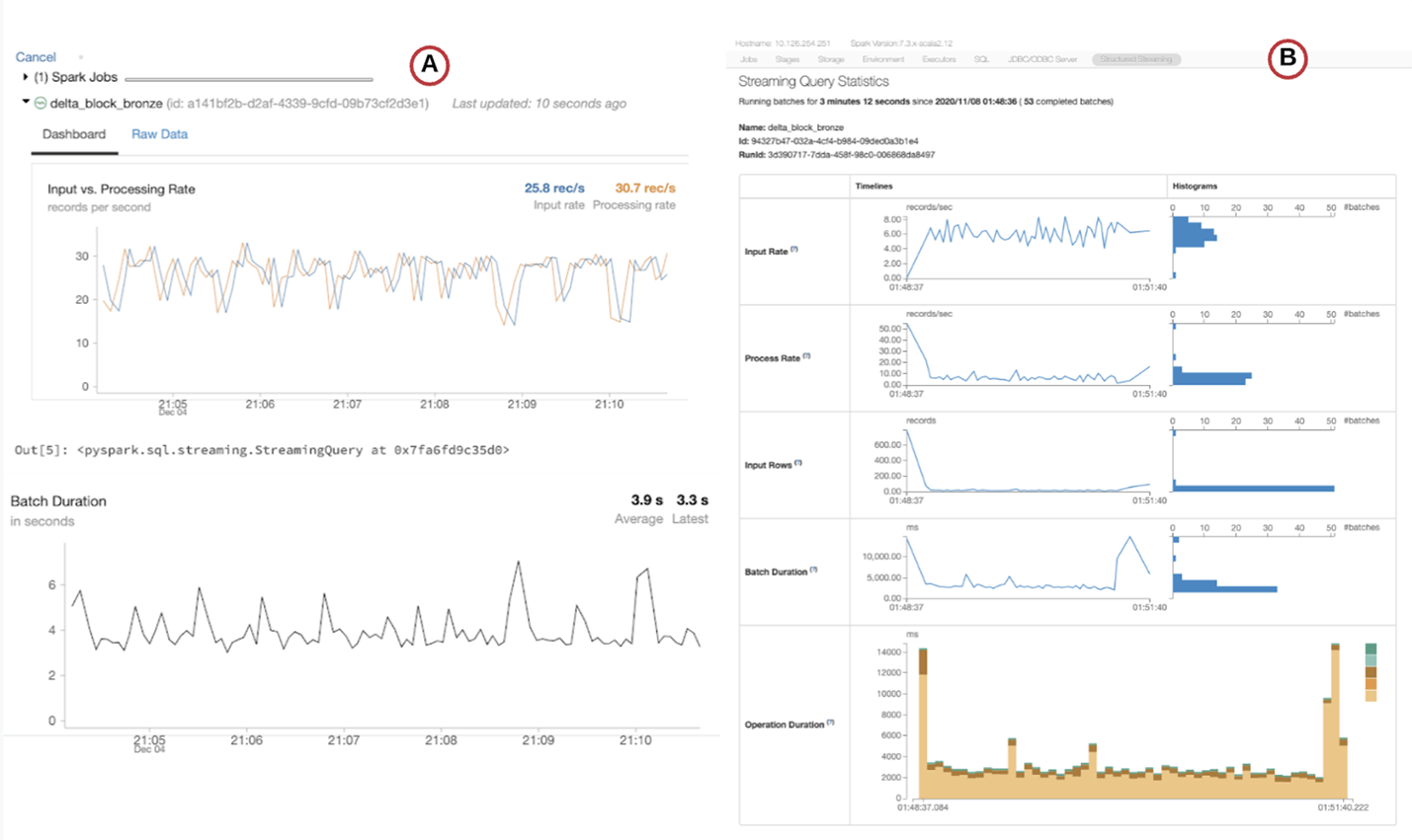
Figure 5: (A) Live Graph and (B) Streaming Query Statistics tab in the Spark UI
- The stream is written out in micro-batches into Delta format. A Delta table is created to point to the data location for easy SQL access. Structured Streaming uses checkpoint files to provide resilience to job failures and ‘exactly once’ semantics.
Step 3:Stream refinement
Stream from the bronze table, flatten the transactions and persist the transaction stream into the silver table.
- ‘round’ is the block number.
- ‘timestamp’ is when committed.
Step 4: In-stream aggregations
Compute in-stream aggregations and persist into the ‘gold’ Delta table.
- Read from the silver Delta table as a streaming job.
- Compute aggregation statistics on transaction data over a sliding window on tx_time. An interval of one hour specifies the aggregation time unit. The watermark allows late arriving data to be included in the aggregates. In distributed and networked systems, there’s always a chance for disruption, which is why it is necessary to preserve the state of the aggregate for a little longer. (keeping it indefinitely will exceed memory capacity)
- Persist into the gold Delta table
Step 5a: Graph analysis
A graph is an intuitive way to model data to discover inherent relationships. With SQL, single hop relations are easy to identify, and graphs are better suited for more complex relationships. This notebook leverages graph processing on the transaction data. Sometimes it is necessary to push data to a specialized graph database. With Spark, it is possible to use the Delta Lake data by applying Graph APIs directly. The notebook utilizes Spark’s distributed computing with the Graph APIs’ flexibility, augmented with additional ML models - all from the same source of truth.
While Blockchain reduces the potential for fraud, there is always a risk of fraud, and Graph semantics can help discover indicative features. Properties of a transaction other than the sender/receiver account ids are more useful in detecting suspicious patterns. A single actor can shield behind multiple identities on the blockchain. For example, a fanout from a single account to multiple accounts through several other layers of accounts and a subsequent convergence to a target account where the original source and target accounts are distinct but in reality map to the same user.
- Create an optimized Delta table for the graph analysis Z-ordered by sender & receiver
- Create Vertices, Edges and construct the transaction Graph from it
- Once the graph is in memory, analyze user activity such as:
- PageRank measures the importance of a vertex (i.e., account) using the directed edges’ link analysis. It is implemented either with controlled iterations or allowing it to converge.
- SP745JJR4KPRQEXJZHVIEN736LYTL2T2DFMG3OIIFJBV66K73PHNMDCZVM was on top of the list. Investigation shows this account processes asset exchanges, which explains the high activity.
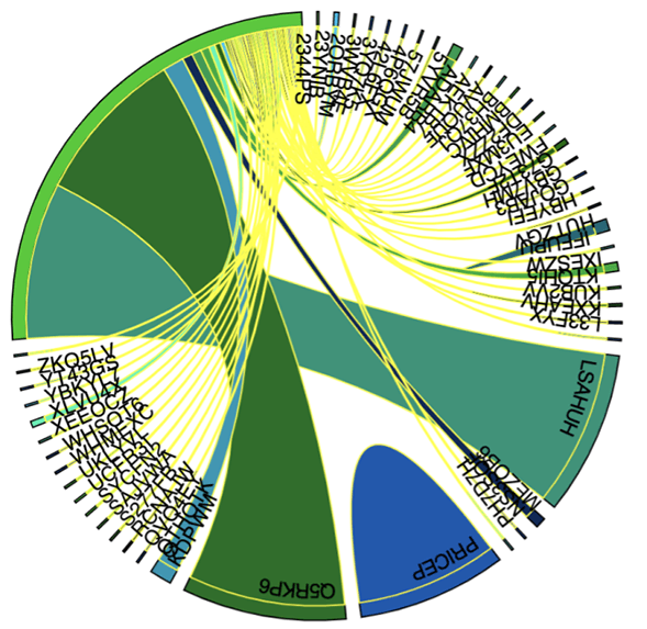 |
D3 chord visualization right inside the Databricks notebook can help show relationships, especially fan-out/in type transactions, using the top active accounts.
The notebook converts the graph tx data into an NxN adjacency matrix, and each vertex is assigned a unique color along the circumference. The chart uses the first 6 char of the account ids for readability. |
Figure 6: Account Interaction using D3 Chord
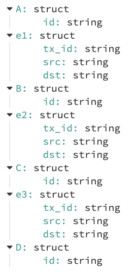
| Motif Search is another powerful search technique to find structural patterns in the graph using a simple DSL (Domain Specific Language).
val motifs_3_hops =
txG.find("(<b>A</b>)-[e1]->(B);(B)-[e2]->(C);(C)-[e3]->(<b>D</b>)")
|
 |
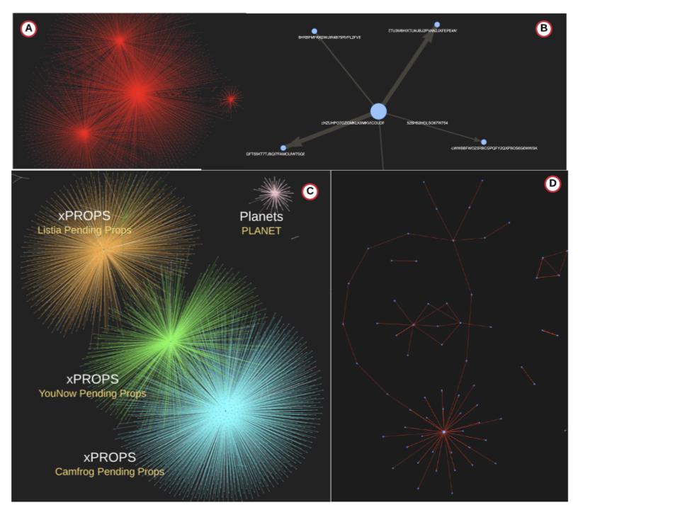
A: Distinct clusters form around the most active accounts.
B: Different types of graphs can be constructed--account to account with the nodes representing the accounts and edges representing the transactions. These are directed graphs with the arrows going from sender to receiver. The thickness of the edge is an indication of the volume of traffic.
C: Another method would involve giving each asset a different color to see how the various assets interact. The diagram above shows a subset of the assets and the observation is that they are generally distinct with some overlap.
D: Zooming into the vortex displays the account id, which aligns with the top senders from the Graph APIs.
Step 5b: SQL Analytics
SQL Analytics offers a performant and full-featured SQL-native query editor that allows data analysts to write queries in a familiar syntax and easily explore Delta Lake table schemas. Queries can be saved in a catalog for reuse and are cached for quicker execution. These queries can be parameterized and set to refresh on an interval and are the building blocks of dashboards that can be created quickly and shared. Like the queries, the dashboards can also be configured to automatically refresh with a minimum refresh interval of a minute and alert the team to meaningful changes in the data. Tags can be added to queries and dashboards to organize them into a logical entity.
The dashboard is divided into multiple sections and each has a different focus:
1. High-level blockchain stats Provides a general overview of key aggregate metrics indicating the health of the blockchain.
2. Algo Price and Volume Monitors the Algo cryptocurrency price and volume for correlation with blockchain stats.
3. Latest (‘Last’) block status Provides stats of the most recent block, which is an indicator of the operational state of the blockchain.
4. Block Trends Provide a historical view of the number of transactions per block and the time required to produce each block.
5. Transaction Trends Provides a more detailed analysis of transaction activity, including volume, transaction type, and assets transferred.
6. Account Activity Provides a view of account behavior, including the most active accounts and the assets transferred between them.
Section 1: High-level blockchain stats
This section is a birds-eye view of aggregate stats, including the count of distinct asset types, transaction types, active accounts in a given time period.
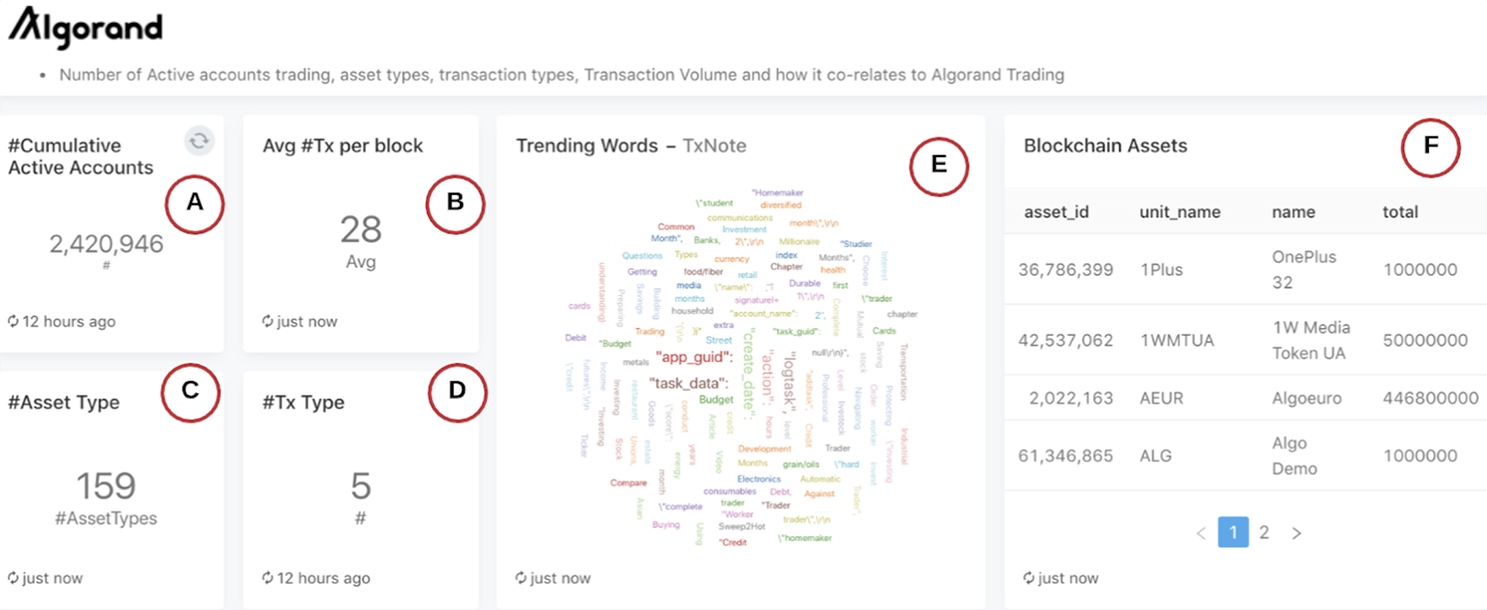
Figure 8: High-level details of the Algorand Blockchain
A: The cumulative number of active accounts in a given time period
B: The average number of transactions per block in the given time period
C: The cumulative number of distinct assets used in the given time period
D: The cumulative number of distinct transaction types in the given time period
E: A word cloud representing the top trending words extracted from the note field of the transactions
F: An alphabetic listing of the asset types. Each asset has a unique identifier, a unit name, and the total number of assets available.
Section 2: Algo price and volume
This section provides price and volume data for Algos, the Algorand cryptocurrency. The price and volume are retrieved using the CryptoCompare API to correlate with the transaction volume.
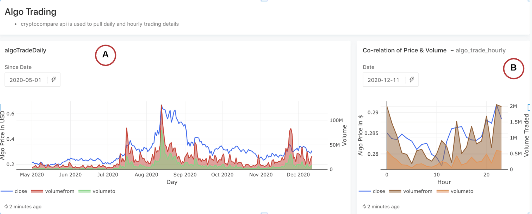
Figure 9: Price and Volume data for Algos
A: Shows trading details daily (Algo price on left axis and volume traded on right axis) since a given date
B: Shows the same on an hourly basis for a given day
Section 3: Latest (‘Last’) block status
The latest block stats are an indicator of the operational state of the blockchain. E.g., suppose the number of transactions in a block or the amount of time it takes to generate a block falls below acceptable thresholds. In that case, it could indicate that the underlying blockchain nodes may not be functioning optimally.
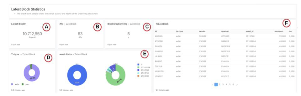
A: The latest Block number
B: Number of transactions in the most recent block
C: Time in seconds for the block to be created
D: The distribution of transaction types in this block
E: The asset type distribution for each transaction type within this block. Pay transactions use Algo and are not associated with an asset type.
F: The individual transactions within this block
Section 4: Block trends
This section is an extension of the previous and provides the historical view of the number of transactions per block and the time required to produce each block.
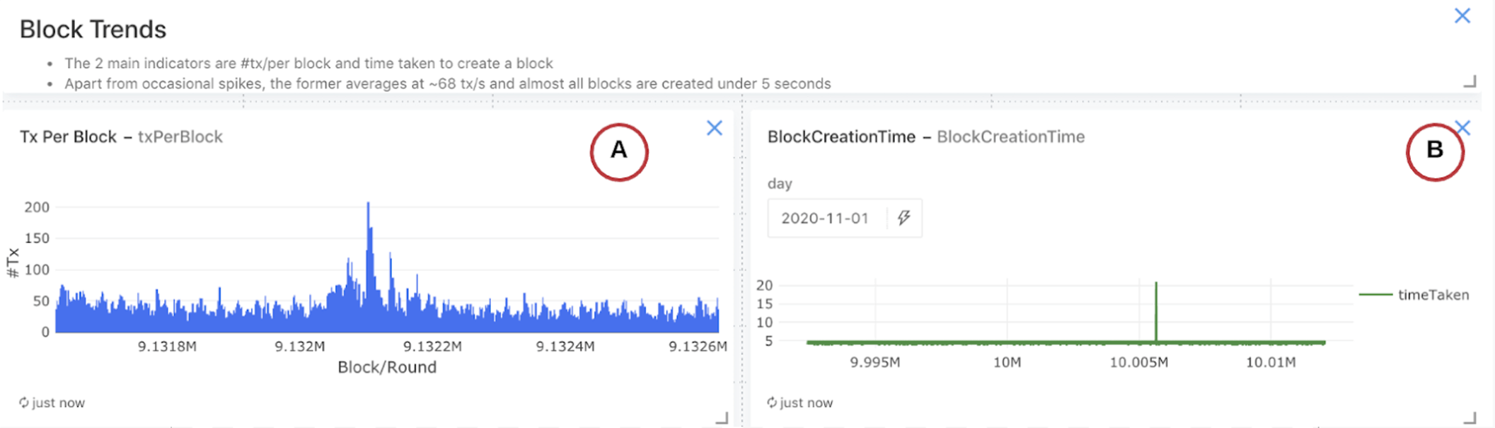
Figure 11: Per block trends
A: The number of transactions per block has a few spikes but shows a regular pattern. Transaction volume is significant since it reflects user adoption on the Algorand blockchain.
B: The time in seconds to create a new block is always less than 5 seconds. The latency indicates the health of the blockchain network and the efficiency of the consensus protocol. An alert monitors this critical metric to ensure that it remains below 5 seconds.
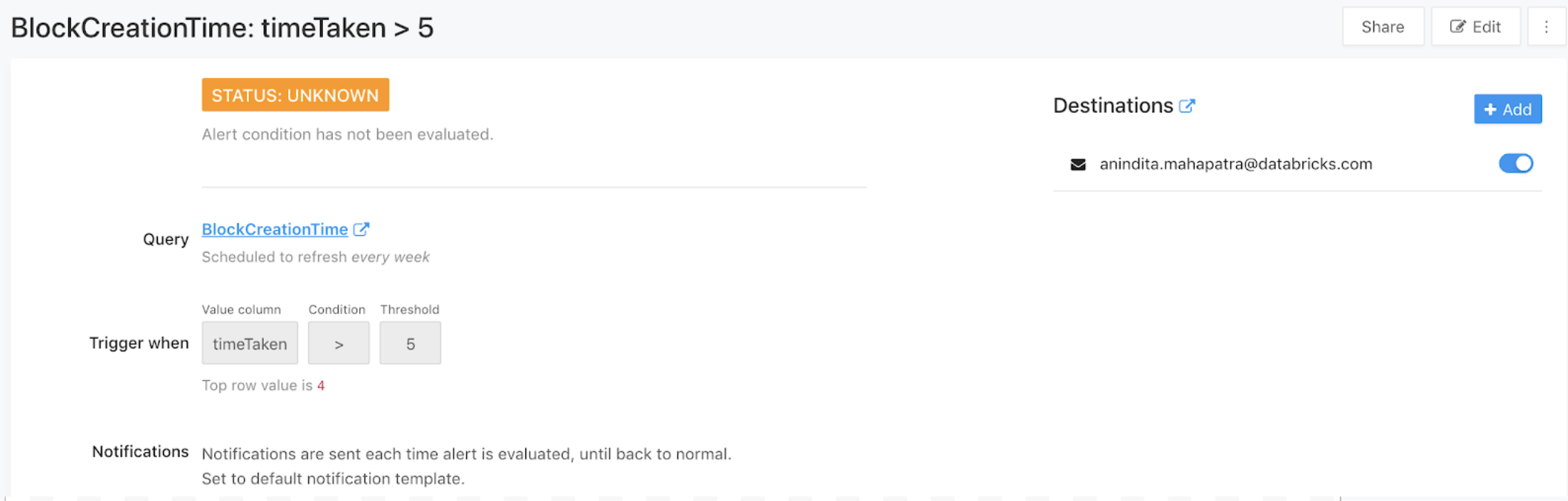
Figure 12: Configuring thresholds for Alert notifications
Section 5: Transactions trends
This section provides a more detailed analysis of transaction activity, including volume, transaction type and assets transferred.
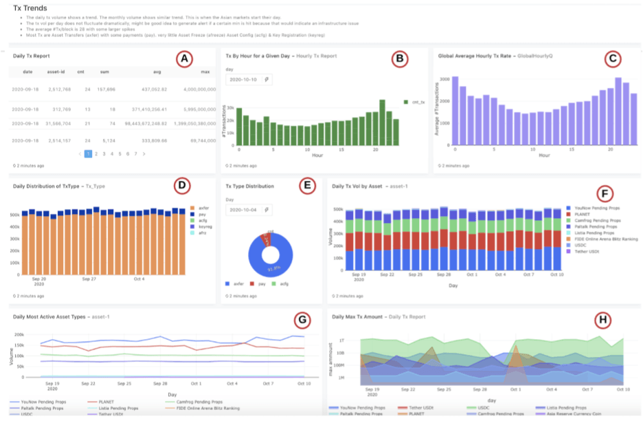
Figure 13: Trends in Transactions
A: Asset statistics (count, average, min, max, sum on the amount) by hour and asset type
B: For a given day, the trend of the transaction count by hour
C: Average transaction volume by hour across the entire time period. There is a pattern that is similar to the previous. It appears that 10 AM is the trough and hour 21 is the crest, possibly on account of Asia’s market waking up.
D: The distribution of transaction types on a daily basis shows a high number of asset transfers (axfer) followed by payments with Algos (pay)
E: The transaction type distribution is the same for the selected day
F: The transaction volume distribution by asset type
G: The transaction volume by asset id over time on a daily basis. YouNow and Planet are the top asset ids traded in the given period.
H: The max transaction amount by asset id over time on a daily basis
Section 6: Account activity
This section provides a view of current account activity, including the most active accounts and the assets transferred. A Sanky diagram illustrates the flow of assets between the most active accounts.
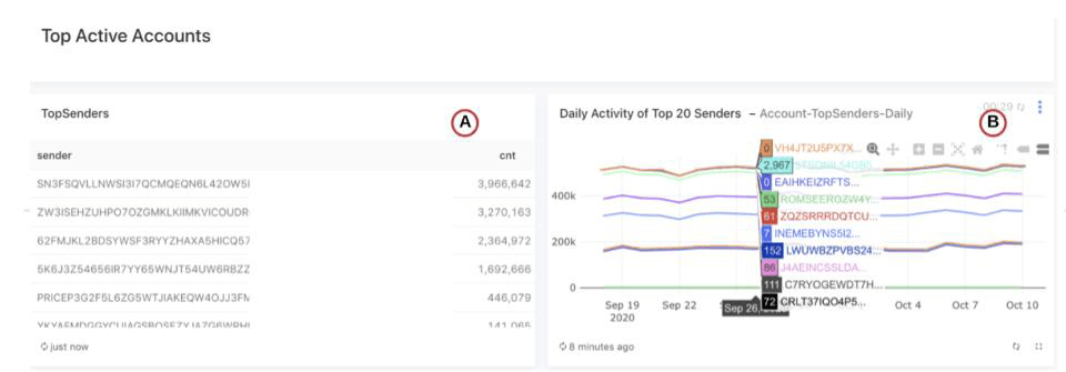
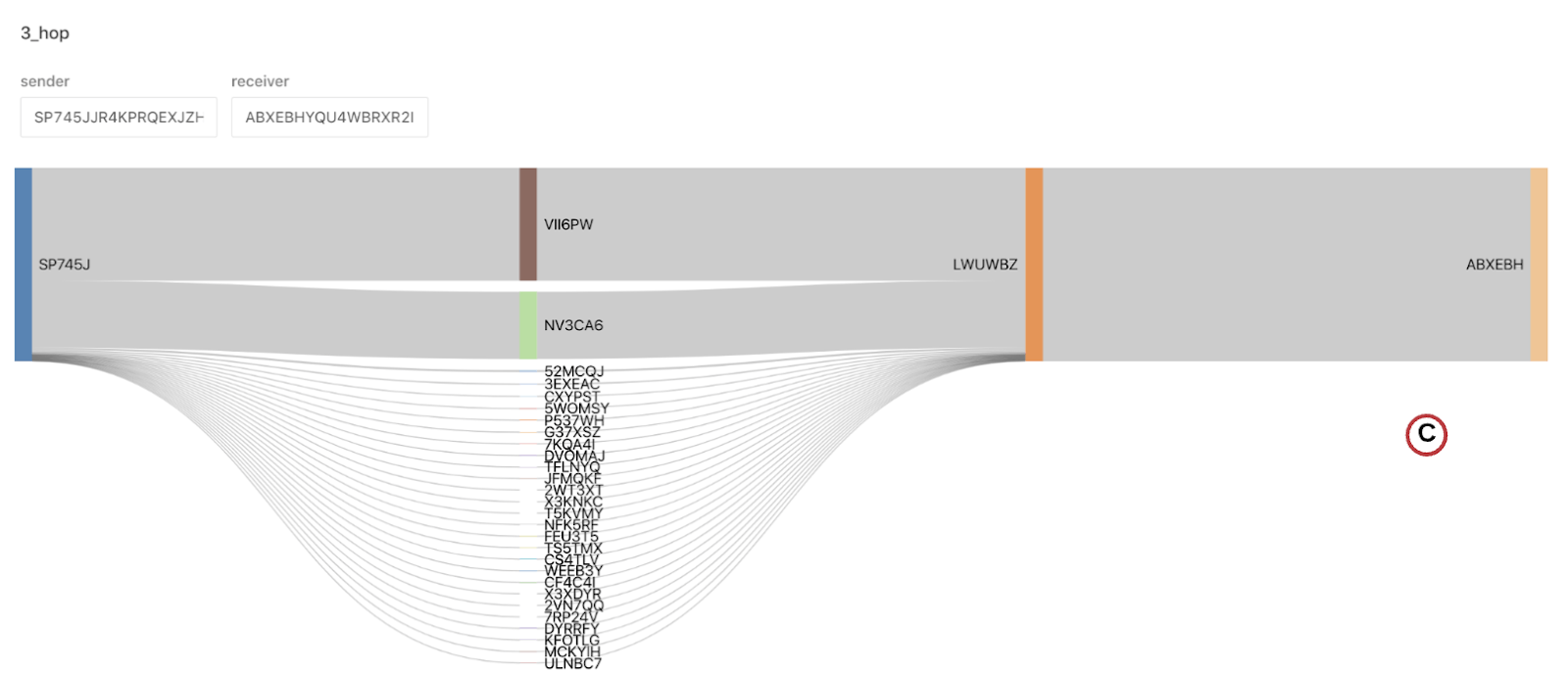
Figure 14: Top Accounts by transaction volume
A: Top Senders by transaction volume
B: Daily transaction volumes of the identified top 20 senders
C: Sankey Diagrams are useful to capture behavioral flows and sequences. Transactions have a ‘point in time view’ of a single sender and receiver. How the transactions flow on either side tell the bigger story and help us understand the hidden nuances of a large source or sink account and contributors along the path.
Summary
This post has shown the Databricks platform's versatility for analyzing transactional blockchain data (block, transaction and account) from the Algorand blockchain in real time. Apache Spark’s open source distributed compute architecture and Delta provide a scalable cloud infrastructure performant with reliable and real-time data streaming and curation. Machine learning practitioners and data analysts perform multiple types of analysis on all the data on a single platform in place. SQL, Python, R and Scala provide the tools for exploratory data analysis. Graph algorithms are applied to analyze account behavior. With SQL Analytics, business analysts derive better business insights through powerful visualizations using queries directly on the data lake.
Try the notebooks
Get the latest posts in your inbox
Subscribe to our blog and get the latest posts delivered to your inbox.