Advertising Fraud Detection at Scale at T-Mobile
by Eric Yatskowitz and Chuong Phan
This is a guest authored post by Data Scientist Eric Yatskowitz and Data Engineer Phan Chuong, T-Mobile Marketing Solutions.
The world of online advertising is a large and complex ecosystem rife with fraudulent activity such as spoofing, ad stacking and click injection. Estimates show that digital advertisers lost about $23 billion in 2019, and that number is expected to grow in the coming years. While many marketers have resigned themselves to the fact that some portion of their programmatic ad spend will go to fraudsters, there has also been a strong pushback to try to find an adequate solution to losing such large sums of advertising money.
This blog describes a research project developed by the T-Mobile Marketing Solutions (TMS) Data Science team intended to identify potentially fraudulent ad activity using data gathered from T-Mobile network. First, we present the platform architecture and production framework that support TMS’s internal products and services. Powered by Apache Spark™ technologies, these services operate in a hybrid of on-premise and cloud environments. We then discuss best practices learned from the development of our Advertising Fraud Detection service, and give an example of scaling a data science algorithm outside of the Spark MLlib framework. We also cover various Spark optimization tips to improve product performance and utilization of MLflow for tracking and reporting, as well as challenges we faced while developing this fraud prevention tool.
Overall architecture
Tuning Spark for ad fraud prevention
Sharing an on-prem Hadoop environment
Working in an on-premise Hadoop environment with hundreds of users and thousands of jobs running in parallel has never been easy. Unlike in cloud environments, on-premise resources (vCPUs and memory) are typically limited or grow quite slowly, requiring a lot of benchmarking and analyzing of Spark configurations in order to optimize our Spark jobs.
Resource management
When optimizing your Spark configuration and determining resource allocation, there are a few things to consider.
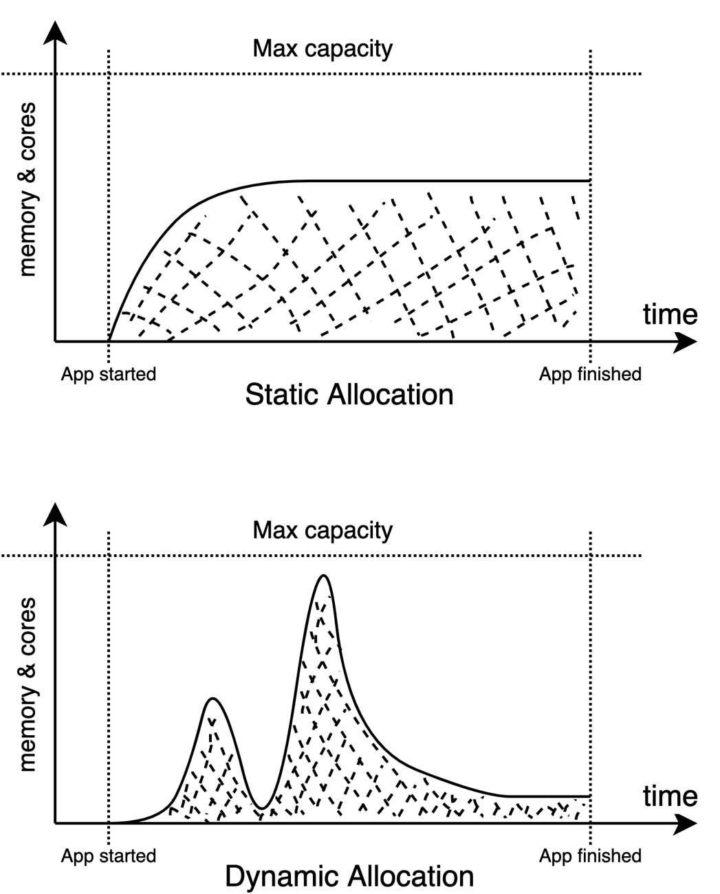
Spark applications use static allocation by default, which means you have to tell the Resource Manager exactly how many executors you want to work with. The problem is you usually don’t know how many executors you actually need before running your job. Often, you end up allocating too few (which makes your job slow, and likely to fail) or too many (so you’re wasting resources). In addition, the resources you allocate are going to be occupied for the entire lifetime of your application, which leads to unnecessary resource usage if demand fluctuates. That’s where the flexible mode called dynamic allocation comes into play. With this mode, executors spin up and down depending on what you’re working with, as you can see from a quick comparison of the following charts.
This mode, however, requires a bit of setup:
- Set the initial (spark.dynamicAllocation.initialExecutors) and minimum (spark.dynamicAllocation.minExecutors) number of executors. It takes a little while to spin these up, but having them available will make things faster when executing jobs.
- Set the maximum number of executors (spark.dynamicAllocation.maxExecutors) because without any limitation, your app can take over the entire cluster. Yes, we mean 100% of the cluster!
- Increase the executor idle timeout (spark.dynamicAllocation.executorIdleTimeout) to keep your executors alive a bit longer while waiting for a new job. This avoids a delay while new executors are started for a job after existing ones have been killed by idling.
- Configure the cache executor idle timeout (spark.dynamicAllocation.cachedExecutorIdleTimeout) to release the executors that are saved in your cache after a certain amount of time. If you don’t set this up and you cache data often, dynamic allocation is not much better than static allocation.
Reading
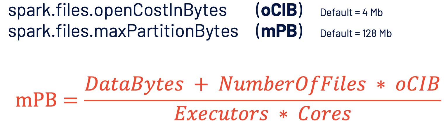
Spark doesn't read files individually; it reads them in batches. It’ll try to merge files together until a partition is filled up. Suppose you have an HDFS directory that has a gigabyte of data with one million files, each with a size of 1 KB (admittedly, an odd use case). If maxPartitionBytes is equal to 8 MB, you will have 500,000 tasks and the job most likely will fail. The chart below shows the correlation between the number of tasks and partition size.
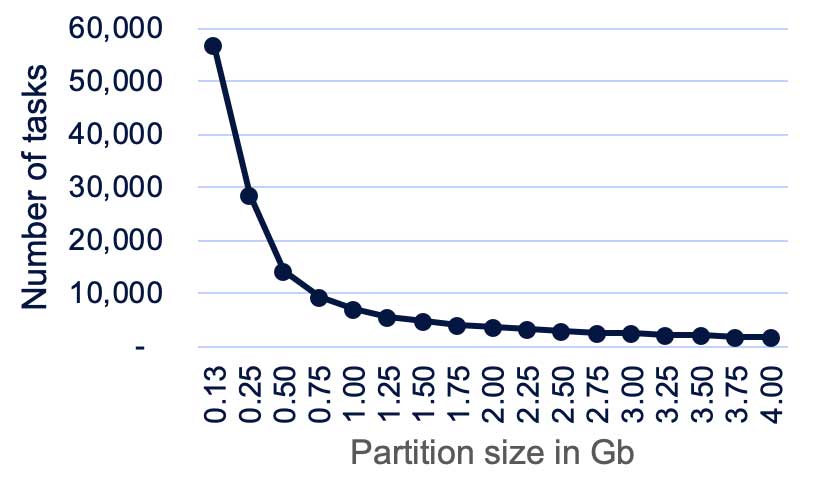
It's quite simple: the bigger the partition you configure, the fewer tasks you will have. Too many tasks might make the job fail because of driver memory error limitations, memory errors, or network connection errors. Too few tasks normally will slow down your job because of lacking parallelization, and quite often it will cause an executor memory error. Fortunately, we’ve found a formula that can calculate the ideal partition size. Plugging in the parameters from the above example will give you a recommended partition size of about 2 GB and 2,000 tasks, a much more reasonable number:
Joining and aggregating
Whenever you join tables or do aggregation, Spark will shuffle data. Shuffling is very expensive because your entire dataset is sent across the network between executors. Tuning shuffle behavior is an art. In the below toy example, there’s a mismatch between the shuffle partition configuration (4 partitions) and the number of currently available threads (8 as a result of 2 cores per executor). This will waste 4 threads.
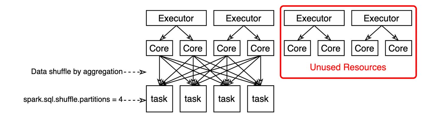
The ideal number of partitions to use when shuffling data (spark.sql.shuffle.partitions) can be calculated by the following formula: ShufflePartitions = Executors * Cores. You can easily get the number of executors if you’re using static allocation, but how about with dynamic allocation? In that case, you can use maxExecutors, or, if you don’t know what the max executor configuration is, you can try using the number of subdirectories of the folder you’re reading from.
Writing
Writing in Spark is a bit more interesting. Take a look at the example below. If you have thousands of executors, you will have thousands of files. The point is, you won’t know if that’s too many or too few files unless you know the data size.
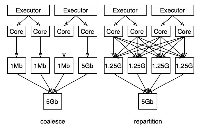
From our experience with huge data, keeping file sizes below 1 GB and the number of files below 2,000 is a good benchmark. To achieve that, you can use either coalesce or repartition:
- The coalesce function works in most cases if you just want to scale down the files, and it’s typically faster because of no data shuffling.
- The repartition function, on the other hand, does a full shuffle and redistributes the data more or less evenly. It will speed up the job if your data is skewed, as in the following example. However, it’s more expensive.
Python to PySpark
Similarities between Python and PySpark
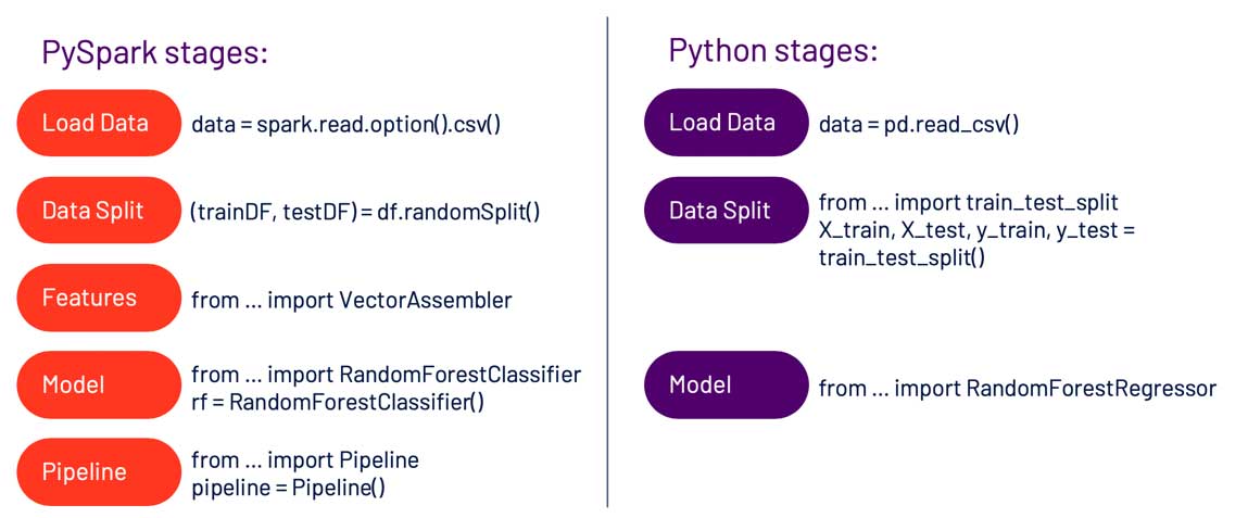
For day-to-day data science use cases, there are many functions and methods in Spark that will be familiar to someone used to working with the Pandas and scikit-learn libraries. For example, reading a CSV file, splitting data into training and test sets, and fitting a model all have similar syntax.
If you’re using only predefined methods and classes, you may not find writing code in Spark very difficult—but there are a number of instances where converting your Python knowledge into Spark code is not straightforward. Whether because the code for a particular machine learning algorithm isn’t in Spark yet or because the code you need is highly specific to the problem you are trying to solve, sometimes you will have to write your own Spark code. Note that if you’re comfortable working with Pandas, Koalas could be a good option for you, as the API works very similarly to how you would work with dataframes in native Python.Take a look at this 10-minute intro to Koalas for more info.
Python UDF vs. PySpark
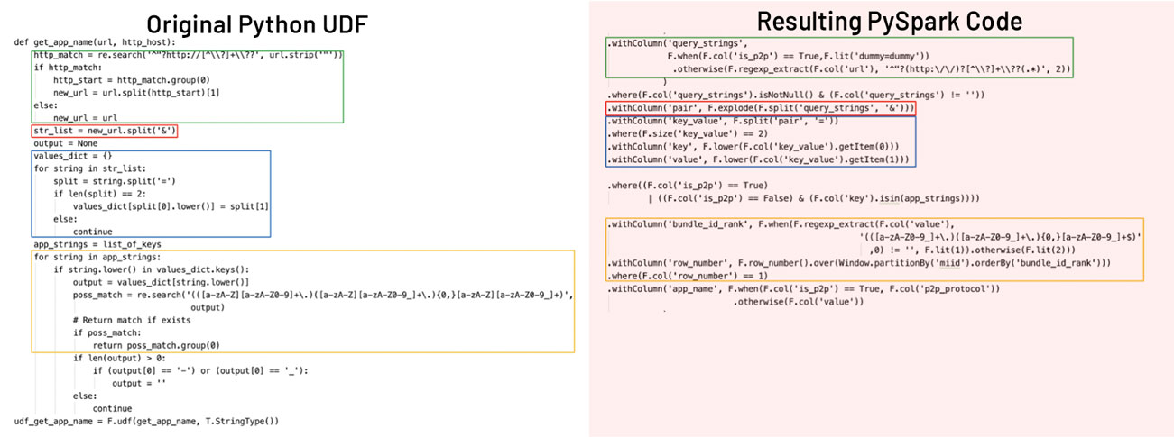
If you’re more comfortable writing code in Python than Spark, you may be inclined to start by writing your code as a Python UDF. Here’s an example of some code we first wrote as a UDF, then converted to PySpark. We started by breaking it down into logical snippets, or sections of code that each perform a fairly basic task, as shown by the colored boxes. This allowed us to find the set of functions that accomplished those tasks. Once they’d been identified, we just had to make sure the bits of code fed into each other and test that the end result was more or less the same. This left us with code that ran natively in Spark rather than a Python UDF.
And to justify this effort, here are the results showing the difference in performance between the UDF and the PySpark code.
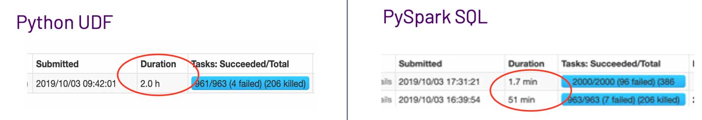
The PySpark code ran over twice as fast, which for a piece of code that runs every day adds up to many hours of compute time savings over the course of the year.
Normalized Entropy
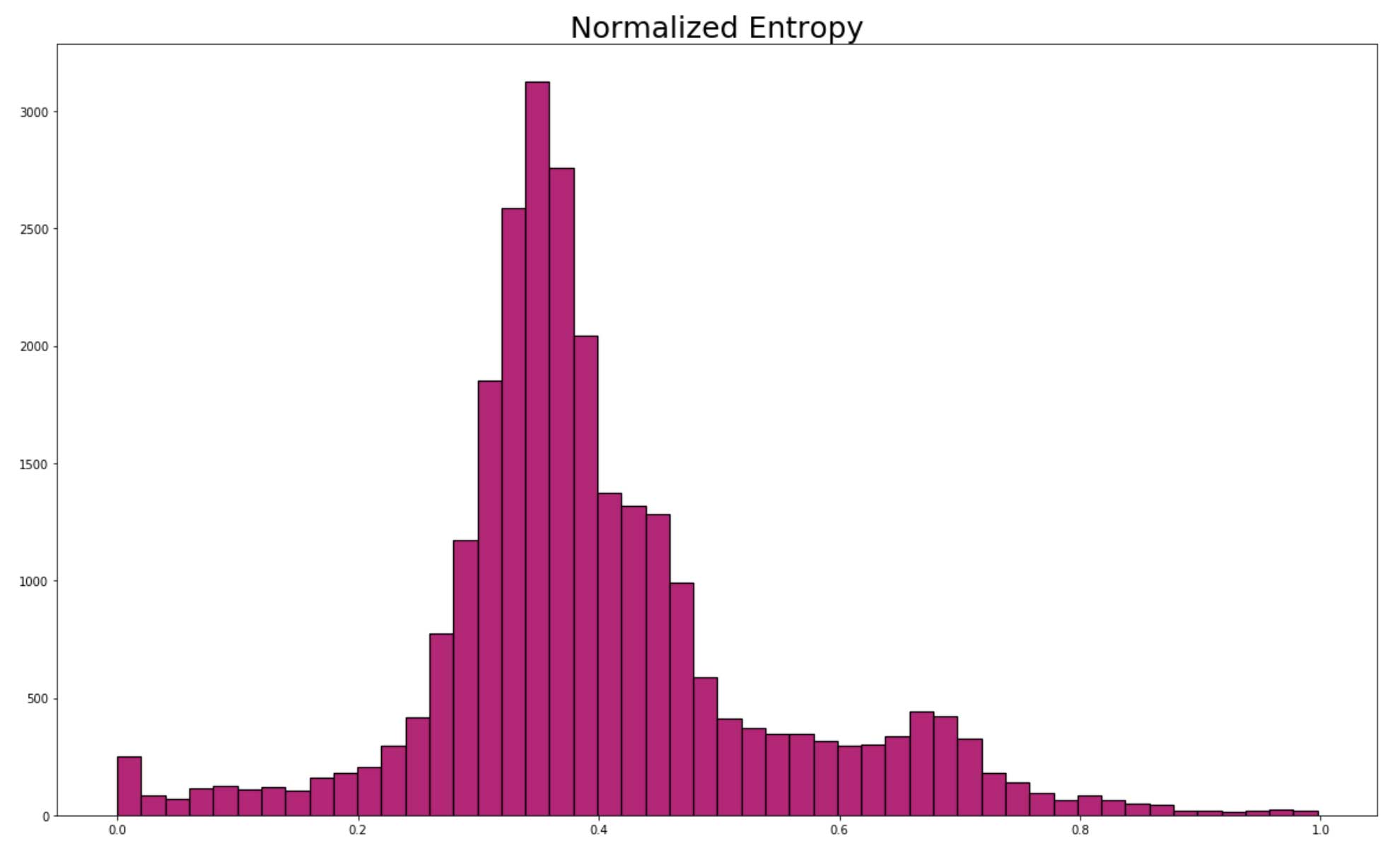
Now, let’s walk through one of the metrics we use to identify potentially fraudulent activity in our network. This metric is called normalized entropy. Its use was inspired by a 2016 paper that found that domains and IPs with very high or low normalized entropy scores based on user traffic were more likely to be fraudulent. We found a similar distribution of normalized entropy scores when analyzing apps using our own network traffic (see the histogram below).
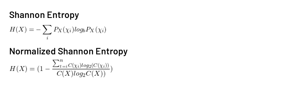
Data scientists familiar with decision trees may know of Shannon entropy, which is a metric commonly used to calculate information gain. The normalized entropy metric we use is the normalized form of Shannon entropy. For those unfamiliar with Shannon entropy, here’s the equation that defines it, followed by the definition of normalized Shannon entropy:
The idea behind this metric is fairly simple. Making the assumption that most apps used by our customers are not fraudulent, we can use a histogram to determine an expected normalized entropy value. Values around the mean of about 0.4 would be considered “normal.” On the other hand, we would score values close to 0 or 1 higher in terms of their potential fraudulence because they are statistically unusual. In addition to the unusualness of values close to 0 or 1, the meaning behind these values is also relevant. A value of 0 indicates that all of the network traffic for that particular app came from a single user, and a value of 1 means multiple users used an app only once. This is of course not a flawless metric—for example, people often only open their banking apps once every few days, so apps like these will have a higher normalized entropy but are unlikely to be fraudulent. Thus, we include several other metrics in our final analysis too.
Static vs. dynamic (revisited)
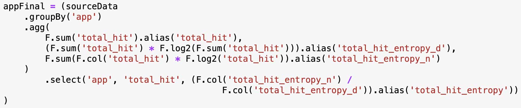
Here is the code we are currently using to calculate normalized entropy:
The last row in the table below shows the time difference between running this code with a default configuration and an optimized configuration. The optimized config sets the number of executors to 100, with 4 cores per executor, 2 GB of memory, and shuffle partitions equal to Executors * Cores--or 400. As you can see, the difference in compute time is significant, showing that even fairly simple Spark code can greatly benefit from an optimized configuration and significantly reduce waiting time. This is a great skill to have for all data scientists who are analyzing large amounts of data in Spark.
Default vs. “optimized” static configuration
| Config | Default | Optimized |
| spark.executors.instances | 2 | 100 |
| spark.executor.cores | 1 | 4 |
| spark.executor.memory | 1g | 2g |
| spark.sql.shuffle.partitions | 200 | 400 |
| Completion time | 8 min | 23 sec |
Finally, let’s chat about the difference between static and dynamic allocation. The two previous configs were static, but when we use dynamic allocation with the same optimized config (shown below), it takes almost twice as long to compute the same data. This is because the Spark cluster initially only spins up the designated minimum or initial number of executors and increases the number of executors, as needed, only after you start running your code. Because executors don’t spin up immediately, this can extend your compute time. This concern is mostly relevant when running shorter jobs and when executing jobs in a production environment, Though, if you’re doing EDA or debugging, dynamic allocation is probably still the way to go.
“Optimized” dynamic configuration
| Config | Default | Optimized |
| spark.dynamicAllocation.maxExecutors | infinity | 100 |
| spark.executor.cores | 1 | 4 |
| spark.executor.memory | 1g | 2g |
| spark.sql.shuffle.partitions | 200 | 400 |
| Completion time | -- | 41 sec |
Productionization
Architecture overview
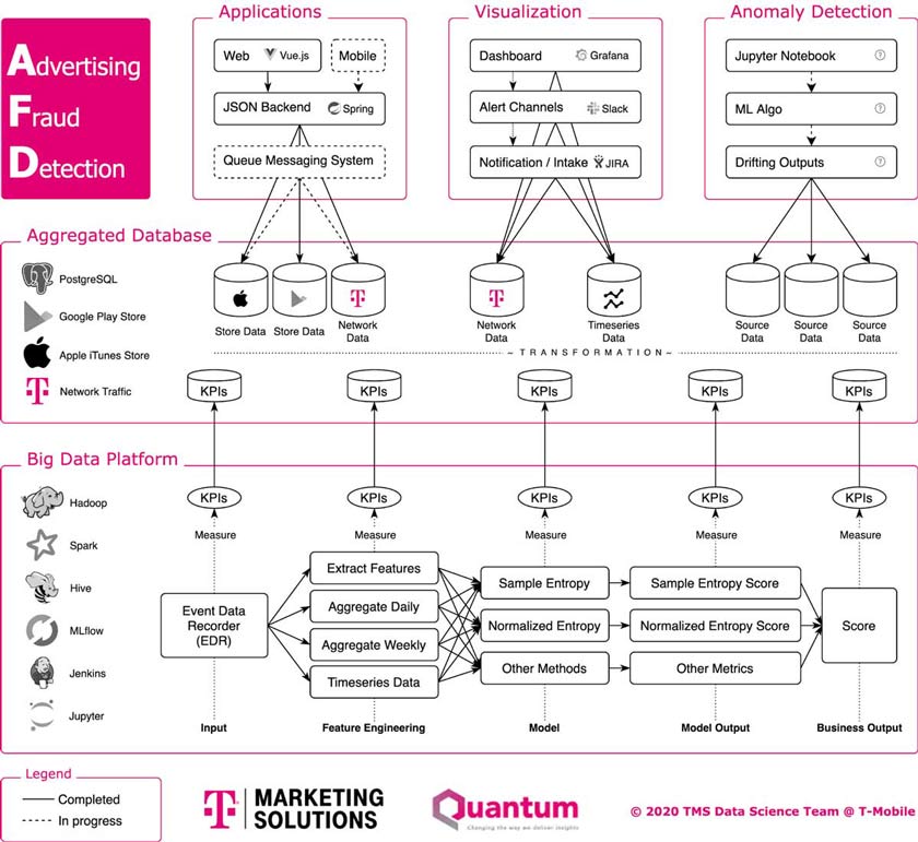
The following image gives an overview of our AdFraud prevention platform. The data pipeline at the bottom of this architecture (discussed in the previous section) is scheduled and put into our Hadoop production environment. The final output of the algorithm and all the other measurements are aggregated and sent out of the Hadoop cluster for use by web applications, analytic tools, alerting systems, etc. We’ve also implemented our own anomaly detection model, and together with MLflow have a complete workflow to automate, monitor and operate this product.
MLflow
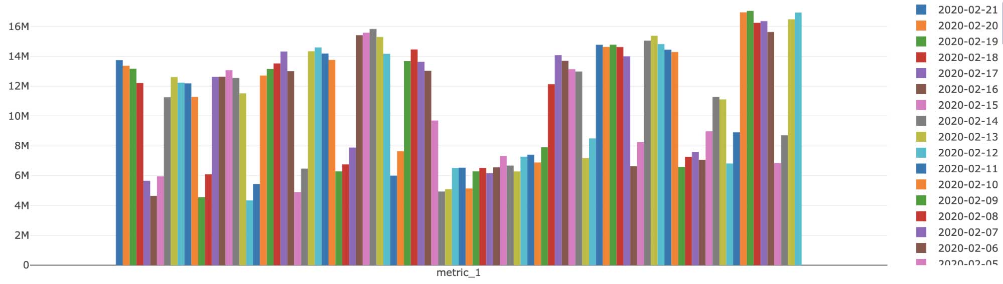
MLflow plays an important role in the monitoring phase because of its simplicity and built-in functions for tracking and visualizing KPIs. With these few lines of code, we are able to log hundreds of our metrics with very little effort:
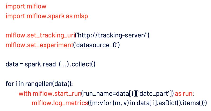
We tag them by dates for visualization purposes, and with an anomaly detection model in place, we’re able to observe our ML model’s output without constant monitoring.
Discussion
As you may know, validation is a very difficult process when it comes to something like ad fraud detection due to the lack of a clear definition of fraud, and it is very important from a legal and moral standpoint to make sure it is done correctly. So, we’re currently working with our marketing team to run A/B tests to validate our process and make improvements accordingly. Advertising fraud is a problem that will not go away on its own. It’s going to take a lot of effort from a variety of different stakeholders and perspectives to keep fraudsters in check and meet the goal of ensuring digital advertising spend is used for its intended purpose.
We’ve provided some details on one approach to attempting to solve this problem using Spark and T-Mobile’s network data. There are a number of alternatives, but regardless of the approach, it’s clear that a very large amount of data will need to be monitored on an ongoing basis—making Spark an obvious choice of tool.
As you’ve seen, optimizing your configurations is key—and not just for the initial reading of your data, but for aggregating and writing as well. Learning to tune your Spark configuration will undoubtedly save you hours of expensive compute time that would otherwise be spent waiting for your code to run.
What's next
Want to learn more or get started with your own use case on Databricks? Contact us to schedule a meeting or sign up for a free trial to get started today.
Get the latest posts in your inbox
Subscribe to our blog and get the latest posts delivered to your inbox.