Beyond LDA: State-of-the-art Topic Models With BigARTM

This post follows up on the series of posts in Topic Modeling for text analytics. Previously, we looked at the LDA (Latent Dirichlet Allocation) topic modeling library available within MLlib in PySpark. While LDA is a very capable tool, here we look at a more scalable and state-of-the-art technique called BigARTM. LDA is based on a two-level Bayesian generative model that assumes a Dirichlet distribution for the topic and word distributions. BigARTM (BigARTM GitHub and https://bigartm.org) is an open source project based on Additive Regularization on Topic Models (ARTM), which is a non-Bayesian regularized model and aims to simplify the topic inference problem. BigARTM is motivated by the premise that the Dirichlet prior assumptions conflict with the notion of sparsity in our document topics, and that trying to account for this sparsity leads to overly-complex models. Here, we will illustrate the basic principles behind BigARTM and how to apply it to the Daily Kos dataset.

Why BigARTM over LDA?

As mentioned above, BigARTM is a probabilistic non-Bayesian approach as opposed to the Bayesian LDA approach. According to Konstantin Vorontsov’s and Anna Potapenko’s paper on additive regularization the assumptions of a Dirichlet prior in LDA do not align with the real-life sparsity of topic distributions in a document. BigARTM does not attempt to build a fully generative model of text, unlike LDA; instead, it choosesto optimize certain criteria using regularizers. These regularizers do not require any probabilistic interpretations. It is therefore noted that the formulation of multi-objective topic models are easier with BigARTM.

Overview of BigARTM

Problem statement

We are trying to learn a set of topics from a corpus of documents. The topics would consist of a set of words that make semantic sense. The goal here is that the topics would summarize the set of documents. In this regard, let us summarize the terminology used in the BigARTM paper:

D = collection of texts, each document ‘d’ is an element of D, each document is a collection of ‘n_d’ words (w₀, w₁,...w_d)

W = collection of vocabulary

T = a topic, a document ‘d’ is supposed to be made up of a number of topics

We sample from the probability space spanned by words (W), documents (D) and topics(T). The words and documents are observed but topics are latent variables.

The term ‘n_dw’ refers to the number of times the word ‘w’ appears in the document ‘d’.

There is an assumption of conditional independence that each topic generates the words independent of the document. This gives us

 

p(w|t) = p(w|t,d)

The problem can be summarized by the following equation

 

 

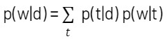
What we are really trying to infer are the probabilities within the summation term, (i.e., the mixture of topics in a document (p(t|d)) and the mixture of words in a topic (p(w|t)). Each document can be considered to be a mixture of domain-specific topics and background topics. Background topics are those that show up in every document and have a rather uniform per-document distribution of words. Domain-specific topics tend to be sparse, however.

 

Stochastic factorization

Through stochastic matrix factorization, we infer the probability product terms in the equation above. The product terms are now represented as matrices. Keep in mind that this process results in non-unique solutions as a result of the factorization; hence, the learned topics would vary depending on the initialization used for the solutions.

We create a data matrix F almost equal to [f_wd] of dimension WxD, where each element f_wd is the normalized count of word ‘w’ in document ‘d’ divided by the number of words in the document ‘d’. The matrix F can be stochastically decomposed into two matrices ∅ and θ so that:

 

F ≈ [∅] [θ]

[∅] corresponds to the matrix of word probabilities for topics, WxT

 

[θ] corresponds to the matrix of topic probabilities for the documents, TxD

All three matrices are stochastic and the columns are given by:

[∅]_t which represents the words in a topic and,

[θ]_d which represents the topics in a document respectively.

The number of topics is usually far smaller than the number of documents or the number of words.

LDA

In LDA the matrices ∅ and θ have columns, [∅]_t and [θ]_d that are assumed to be drawn from Dirichlet distributions with hyperparameters given by β and α respectively.

β= [β_w], which is a hyperparameter vector corresponding to the number of words

α= α[α_t], which is a hyperparameter vector corresponding to the number of topics

Likelihood and additive regularization

The log-likelihood we would like to maximize to obtain the solution is given by the equations below. This is the same as the objective function in Probabilistic Latent Semantic Analysis (PLSA) and will be the starting point for BigARTM.

 

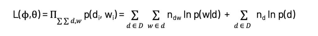
We are maximizing the log of the product of the joint probability of every word in each document here. Applying Bayes Theorem results in the summation terms seen on the right side in the equation above. Now for BigARTM, we add ‘r’ regularizer terms, which are the regularizer coefficients τ_i multiplied by a function of ∅ and θ.

 

 

where R_i is a regularizer function that can take a few different forms depending on the type of regularization we seek to incorporate. The two common types are:

 

1. Smoothing regularization
2. Sparsing regularization

In both cases, we use the KL Divergence as a function for the regularizer. We can combine these two regualizers to meet a variety of objectives. Some of the other types of regularization techniques are decorrelation regularization and coherence regularization. (http://machinelearning.ru/wiki/images/4/47/Voron14mlj.pdf, e.g. 34 and eq. 40.) The final objective function then becomes the following:

 

L(∅,θ) + Regularizer

 

Smoothing regularization

Smoothing regularization is applied to smooth out background topics so that they have a uniform distribution relative to the domain-specific topics. For smoothing regularization, we

1. Minimize the KL Divergence between terms [∅]_t and a fixed distribution β
2. Minimize the KL Divergence between terms [θ]_d and a fixed distribution α
3. Sum the two terms from (1) and (2) to get the regularizer term

We want to minimize the KL Divergence here to make our topic and word distributions as close to the desired α and β distributions respectively.

Sparsing strategy for fewer topics

To get fewer topics we employ the sparsing strategy. This helps us to pick out domain-specific topic words as opposed to the background topic words. For sparsing regularization, we want to:

1. Maximize the KL Divergence between the term [∅]_t and a uniform distribution
2. Maximize the KL Divergence between the term [θ]_d and a uniform distribution
3. Sum the two terms from (1) and (2) to get the regularizer term

We are seeking to obtain word and topic distributions with minimum entropy (or less uncertainty) by maximizing the KL divergence from a uniform distribution, which has the highest entropy possible (highest uncertainty). This gives us ‘peakier’ distributions for our topic and word distributions.

Model quality

The ARTM model quality is assessed using the following measures:

1. Perplexity: This is inversely proportional to the likelihood of the data given the model. The smaller the perplexity the better the model, however a perplexity value of around 10 has been experimentally proven to give realistic documents.
2. Sparsity: This measures the percentage of elements that are zero in the ∅ and θ matrices.
3. Ratio of background words: A high ratio of background words indicates model degradation and is a good stopping criterion. This could be due to too much sparsing or elimination of topics.
4. Coherence: This is used to measure the interpretability of a model. A topic is supposed to be coherent, if the most frequent words in a topic tend to appear together in the documents. Coherence is calculated using the Pointwise Mutual Information (PMI). The coherence of a topic is measured as:
   • Get the ‘k’ most probable words for a topic (usually set to 10)
   • Compute the Pointwise Mutual Information (PMIs) for all pairs of words from the word list in step (a)
   • Compute the average of all the PMIs
5. Kernel size, purity and contrast: A kernel is defined as the subset of words in a topic that separates a topic from the others, (i.e. W_t = {w: p(t|w) >δ}, where is δ selected to about 0.25). The kernel size is set to be between 20 and 200. Now the terms purity and contrast are defined as:

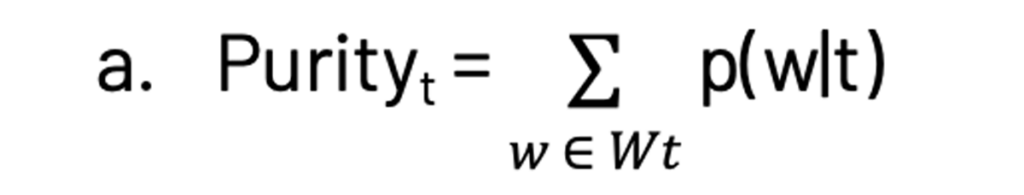
which is the sum of the probabilities of all the words in the kernel for a topic

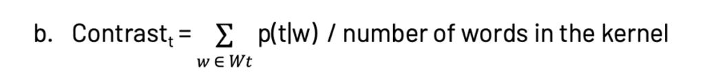
For a topic model, higher values are better for both purity and contrast.

Using the BigARTM library

Data files

The BigARTM library is available from the BigARTM website and the package can be installed via pip. Download the example data files and unzip them as shown below. The dataset we are going to use here is the Daily Kos dataset.

LDA

We will start off by looking at their implementation of LDA, which requires fewer parameters and hence acts as a good baseline. Use the ‘fit_offline’ method for smaller datasets and ‘fit_online’ for larger datasets. You can set the number of passes through the collection or the number of passes through a single document.

You can extract and inspect the ∅ and θ matrices, as shown below.

ARTM

This API provides the full functionality of ARTM, however, with this flexibility comes the need to manually specify metrics and parameters.

You can use the model_artm.get_theta() and model_artm.get_phi() methods to get the ∅ and θ matrices respectively. You can extract the topic terms in a topic for the corpus of documents.

Conclusion

LDA tends to be the starting point for topic modeling for many use cases. In this post, BigARTM was introduced as a state-of-the-art alternative. The basic principles behind BigARTM were illustrated along with the usage of the library. I would encourage you to try out BigARTM and see if it is a good fit for your needs!

Please try the attached notebook.