Anomaly Detection to Prevent Energy Loss

Energy loss in the utility space is primarily broken down into two categories: fraud and leakage. Fraud (or energy theft) is malicious and can range from meter tampering, tapping into neighboring houses, or even running commercial loads on residential property (e.g. grow houses). Meter tampering is traditionally handled by personnel doing routine manual checks, but newer advances in computer vision allow the use of lidar and drones to automate these checks.

Energy leakage is usually thought of in terms of physical leaks, like broken pipes, but can encompass many more prominent issues. For example, a window left open during winter can cause abnormal energy usage in a home powered by a heat pump, or a space heater being accidently left on for multiple days. Each of these situations represents energy loss and should be dealt with accordingly to protect consumers from rising costs and to conserve energy in general, but accurately identifying energy loss at scale can be daunting when taking a human-first approach. The remainder of this article will take a scientific approach to utilize machine learning methods on Databricks to tackle this problem at scale with out-of-the-box distributed compute, built-in orchestration, and end-to-end MLOps.

Detecting Energy Loss At Scale

The initial problem many utility companies face in efforts to detect energy loss is the absence of accurately labeled data. Because of reliance on self reporting from the customer, several issues arise. First, consumers may not realize there is a leak at all. For example, the smell of gas may not be prominent enough from a small leak or a door was left cracked while on vacation. Second, in the case of fraud there is no incentive to report excessive usage. It is hard to pick out theft using simple aggregation because things like weather and home size need to be taken into account to validate abnormalities. Lastly, the manpower required to investigate every report, many of which are false alarms, is taxing on the organization. In order to overcome these types of hurdles, utility companies can utilize data to take a scientific approach with machine learning to detect energy loss.

A Phased Approach to Energy Loss Detection

As described above, the reliance on self-reported data leads to inconsistent and inaccurate results, preventing utility companies from building an accurate supervised model. Instead, a proactive data-first approach should be taken rather than a reactive "report and investigate". Such a data-first approach could be split into three phases: unsupervised, supervised, and maintenance. Starting with an unsupervised approach allows for pointed verification to generate a labeled dataset by detecting anomalies without any training data. Next, the outputs from the unsupervised step can be fed into the supervised training step that uses labeled data to build a generic and robust model. Since patterns in gas and electricity usage change due to consumption and theft patterns, the supervised model will become less accurate over time. In order to combat this, the unsupervised models continue to run as a check against the supervised model.. To illustrate this, an electric meter dataset that contains hourly meter readings combined with weather data will be utilized to construct a rough framework for doing energy loss detection.

Unsupervised Phase

This first phase should serve as a guide for investigating and validating potential loss and should be more accurate than random inspections. The primary goal here is to provide accurate input to our supervised phase, with a short-term goal of reducing the operational overhead of obtaining this labeled data. Ideally, this exercise should start with a subset of the population with as much diversity as possible including factors such as home size, number of floors, age of the home, and appliance information. Even though these factors will not be used as features in this phase, they will be important when building a more robust supervised model in the next phase.

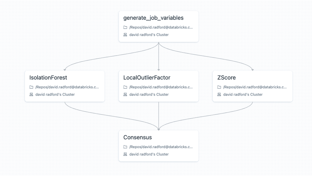
The unsupervised approach will use a combination of techniques to identify anomalies at a meter level. Instead of relying on a single algorithm, it can be more powerful to use an ensemble (or collection of models) to develop a consensus. There are many pre-built models and equations that are useful to identify anomalies ranging from simplistic statistics to deep learning algorithms. For this exercise, three methods were selected: isolation forest, local outlier, and a z-score measurement

The z-score equation is very simplistic and extremely lightweight to compute. It simply takes a value, subtracts the average of all the values, and then divides it by the standard deviation. In this case, the value will represent a single meter reading for a building, the average will be the average of all the readings for that building, and the same with standard deviation.

z = ( x - μ ) / σ

If the score is above three then it is considered an anomaly. This can be a highly accurate way to quickly see the value, but this approach alone will not consider other factors such as weather and time of day.

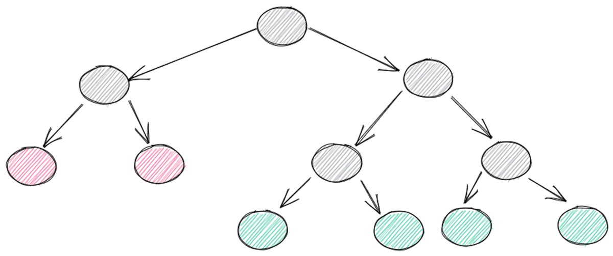
The Isolation forest (iForest) model builds an ensemble of isolation trees where the anomalous points have the shortest traversal path.

The benefit of this approach is that it can be multi-dimensional data, which can add to the accuracy of the predictions. This added overhead can equate to around twice as much runtime as the simple z-score. The hyper-parameters are very few which keeps the tuning to a minimum still.

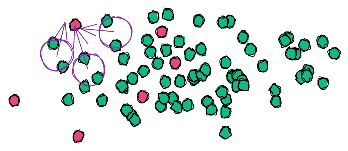
The Local outlier factor (LOF) model uses the density (or distance between points) of a local cluster compared to the density of its neighbors to determine outliers.

LOF has about the same computational needs as iForest but is more robust in detecting localized anomalies rather than global anomalies.

The implementation for each of these algorithms will scale on a cluster using either built-in SQL functions for z-score or a pandas UDF for scikit-learn models. Each model will be applied at an individual meter level to account for unknown variables such as occupant habits.

Z-score uses the formula introduced above and will mark a record as anomalous if the score is greater than three.

select
   building_id,
   timestamp,
   meter_reading,
   (meter_reading - avg_meter_reading) / std_dev_meter_reading as meter_zscore
 from
   raw

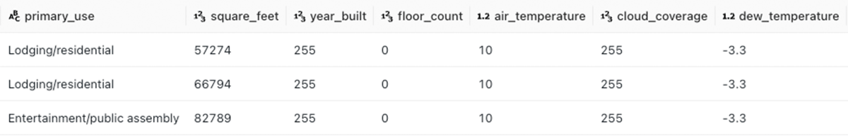
iForest and LOF will both use the same input because they are multi-dimensional models. The use of some key features will produce the best results. In this example, structural features are ignored because they will be static for a given meter. Instead, the focus is placed on air temperature.

df = spark.sql(f"""select building_id,
timestamp,
meter_reading,
ntile(200) over(partition by building_id order by air_temperature) as air_temperature_ntile
from [catalog].[database].raw_features
where meter_reading is not null
and timestamp <= '{cutoff_time}'""")

This is grouped and passed to a pandas UDF for distributed processing. Some metadata columns are added to the results to indicate which model was used and to store the unique ensemble identifier.

results = (
 df.groupBy("building_id")
   .applyInPandas(train_model, schema="building_id int, timestamp timestamp, anomaly int, score double")
   .withColumn("model_name",lit("local_outlier_factor"))
   .withColumn("prediction_time",current_timestamp())
   .withColumn("ensemble_id", lit(ensemble_id))
)

The three models can then be run in parallel using Databricks Workflows. Task values are used to generate a shared ensemble identifier so that a consensus can query data from the same run of the workflow. The consensus step will do a simple majority vote for the three models to determine if it is an anomaly or not.

Models should be run at daily (or even hourly) intervals to identify potential energy loss in order to validate it before the issue goes away or is forgotten by the customer (e.g. I don't remember leaving a window open last week) If possible, all anomalies should be investigated, and even random (or semi-random) sets of normal values should routinely be inspected to ensure anomalies are not slipping through the cracks. Once a few months of iterations have taken place, the properly labeled data can be fed into the supervised model for training.

Supervised Phase

In the previous section, an unsupervised approach was used to accurately label anomalies with the added benefit of detecting potential leaks or theft a few times a day. The supervised phase will use this newly labeled data combined with features like home size, number of floors, age of the home, and appliance information to build a generic model that can proactively detect anomalies as they are ingested. When dealing with larger volumes of data, including several years of historical utility usage at a detailed level, standard ML techniques can become less performant than desired. In such cases, the Spark ML library will take advantage of Spark's distributed processing. Spark ML is a machine learning library that provides a high-level Dataframe-based API that makes ML on Spark scalable and easy. It includes many popular algorithms and utilities as well as the ability to convert ML workflows into Pipelines–more on this in a bit. For now, the goal is just to create a baseline model on our labeled data using a simple logistic regression model.

To start, the labeled dataset is loaded into a dataframe from a Delta table using Spark SQL.

df = spark.sql(f"""select * from [catalog].[database].[table_with_labels] where meter_reading is not null""")

Since the ratio of anomalous records appears to be significantly imbalanced, a balanced dataset is created by taking a sample of the majority class and joining it to the entire minority (anomalies) DataFrame using PySpark.

from pyspark.sql.functions import col
major_df = df.filter(col("anomaly") == 0)
minor_df = df.filter(col("anomaly") == 1)
ratio = int(major_df.count()/minor_df.count())
sampled_majority_df = major_df.sample(False, 1/ratio, seed=12345)
rebalanced_df = sampled_majority_df.unionAll(minor_df)

After dropping some unnecessary columns, the new rebalanced DataFrame is split into train and test datasets. At this point, a pipeline can be built with SparkML using the Pipelines API, similar to the pipeline concept in scikit-learn. A pipeline consists of a sequence of stages that are run in order, transforming the input DataFrame at each stage.

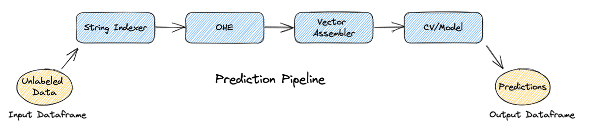
In the training step, the pipeline will consist of four stages: a string indexer and one-hot encoder for handling categorical variables, a vector assembler for creating a required single array column consisting of all features, and cross-validation. From that point, the pipeline can be fit on the training dataset.

stages = [string_indexer, ohe_encoder, vec_assembler, cv]
pipeline = Pipeline(stages=stages)
pipeline_model = pipeline.fit(train_df)

Then, the test dataset can be passed through the new model pipeline to get an idea of accuracy.

pred_df = pipeline_model.transform(test_df)

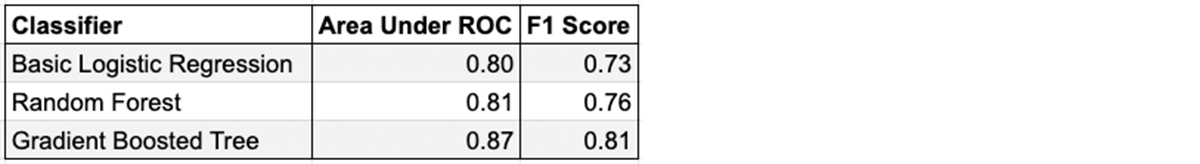
Resulting metrics can be calculated for this basic LogisticRegression estimator.

Area under ROC curve: 0.80
F1 Score: 0.73

A simple change to the estimator used in the cross-validation step will allow for a different learning algorithm to be evaluated. After testing out three different estimators (LogisticRegression, RandomForestClassifier, and GBTClassifier) it was determined that GBTClassifier resulted in slightly better accuracy.

Not bad, given some very basic code with little tuning and customization. To improve model accuracy and productionalize a reliable ML pipeline, additional steps such as enhanced feature selection, hyperparameter tuning, and adding explainability details could be added.

Maintenance Layer

Over time, new scenarios and circumstances contributing to energy loss will occur that the supervised model has not seen before–changes in weather patterns, appliance upgrades, home ownership, and fraud practices. With this in mind, a hybrid approach should be implemented. The highly accurate supervised model can be used to predict known scenarios in parallel with the unsupervised ensemble. A highly confident prediction from the unsupervised ensemble can be used to override the supervised decision to elevate a potential anomaly from edge (or unseen) scenarios. Upon verification, the results can be fed back into the system for re-training and expansion of the supervised model. By using built in orchestration capabilities on Databricks, this solution can be effectively deployed for both real-time anomaly predictions as well as offline checks with the unsupervised models.

Conclusion

Preventing energy loss is a challenging problem that requires the ability to detect anomalies at massive scale. Traditionally it is a problem that can be very difficult to address because it requires a large field initiative for investigation to supplement a very small and often inaccurately-reported dataset. Taking a scientific approach for investigation using unsupervised techniques greatly reduces the manpower required to develop an initial training dataset, which lowers the barrier of entry to develop more accurate supervised models that are custom fit to the population. Databricks provides built-in orchestration of these ensemble models and the necessary capabilities to do distributed model training, removing traditional limitations on data input sizes and enabling the full machine-learning lifecycle at scale.

Learn More