Best Practices for Realtime Feature Computation on Databricks

As Machine Learning usage continues to rise across industries and applications, the sophistication of the Machine Learning pipelines is also increasing. Many of our customers are moving away from using batch pipelines to generate predictions ahead of time and instead opting for realtime predictions. A common question that arises in this context is: "How do I make predictions of the model sensitive to the latest actions of the user?". For many models, this is the key to realizing the greatest business value from switching to a real-time architecture. For example, a product recommendation model that is aware of the products a customer is currently viewing is qualitatively better than a static model.

In this blog, we will examine the most effective architectures for providing real-time models with fresh and accurate data using Databricks Feature Store and MLflow. We will also provide an example to illustrate these techniques.

Feature Engineering at the core of modeling a system

When a data scientist is building a model they are looking for signals that can predict the behavior or outcomes of the complex system. The data signals used as inputs to the ML models are called features. Typically both raw signals coming from live, realtime data sources and aggregated historical features can be predictors of future behavior. Data scientists want to discover existing aggregated features in the Lakehouse and reuse them for other machine learning projects.

When computing these aggregations from raw inputs, a data engineer needs to make tradeoffs across various interrelated dimensions: complexity of the calculation, size of input data, freshness requirements and importance of each signal to the model's prediction, expected latency of online system, cost of feature computation and model scoring. Each of these has significant implications on architecture of the feature computation pipeline and usage in model scoring. One of the most significant drivers amongst these is data freshness and how each signal affects the accuracy of model prediction.

Data freshness can be measured from the time a new event is available to a computation pipeline to the time the computed feature value is updated in batch storage or becomes available for online model inference. In other words, it determines how stale the feature values being used in predictions are. The data freshness requirement captures how quickly the values of the feature change, e.g. if the feature is fast or slow changing.

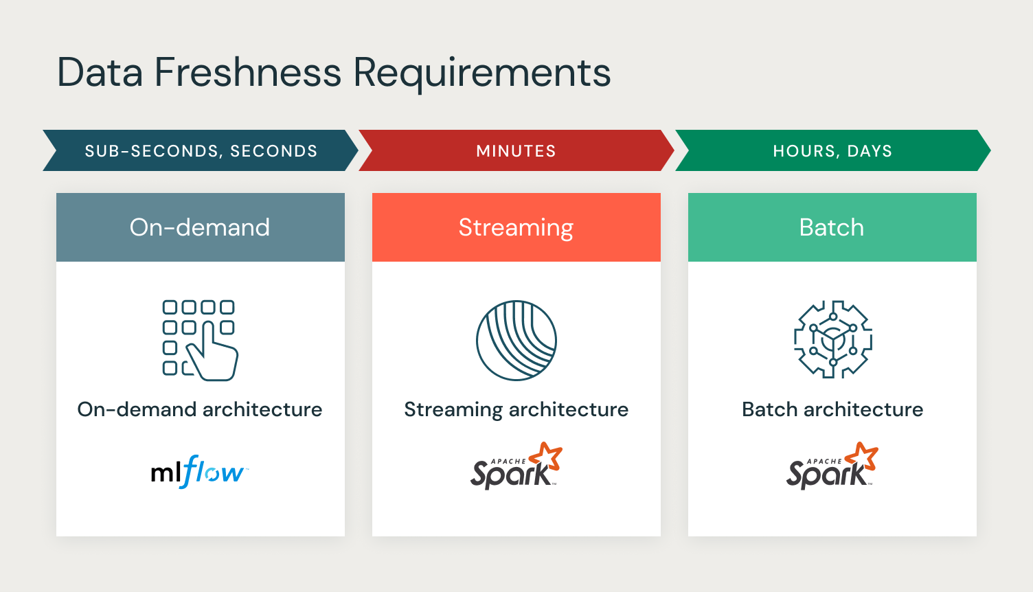
Let's consider how data freshness affects the choices a data engineer makes for feature computation. Broadly there are three architectures to choose from: batch, streaming, on-demand with varying degree of complexity and cost implications.

Computation Architectures for Feature Engineering

Batch computation frameworks (like Spark and Photon) are efficient at computing slowly changing features or features that require complex calculations typically with large volumes of data. With this architecture, pipelines are triggered to pre-compute feature values and materialized in offline tables. They may be published to online stores for low latency access to real-time model scoring. This type of features can be used where data freshness has a lower effect on the model performance. Common examples include statistical features that aggregate a particular metric over time in a product recommendation system using customer's total purchases over their lifetime, or historical popularity of a product.

Data freshness matters more for features whose values are rapidly changing in the real world - feature values can quickly become stale and degrade the accuracy of model predictions. Data scientists prefer to use on-demand computation such that features can be computed from latest signals at the time of models scoring. These will typically use simpler calculations and use smaller raw inputs. Another scenario for using on-demand computation is when features may change their values much more frequently than the values are actually being used in model scoring. Frequently recomputing such features for a large number of objects quickly becomes inefficient and at times cost-prohibitive. For example, in the aforementioned user product viewing history cosine similarity between user preferences and item embeddings of the products viewed in the last 1 minute, percentage of discounted items in that session are all examples of features best computed on-demand.

There are also features that fall in-between these two extremes. The feature may require larger computation or use a high throughput stream of data than can be done on-demand with low latency, but also change values faster than what batch architecture can accommodate. These near real-time features are best computed using streaming architecture, which asynchronously pre-computes feature values similar to batch architecture but does it continuously on a stream of data.

Choosing computation architecture

The good starting point of selecting computational architecture is the data freshness requirement. In simpler cases, when data freshness requirements are not strict, batch or streaming architectures are the first choice. They are simpler to implement, can accommodate big computational needs and deliver predictable low latency. In more advanced cases, when we need to build a model able to react quickly to user behavior or external events, the data freshness requirements become stricter and the on-demand architecture becomes more appropriate to accommodate these requirements.

Now that we have established the general guidance, let's illustrate on the specific example, how Databricks Feature Store and MLflow can be used to implement all three architectures for computation of different types of features.

Example: Ranking model for travel recommendation

Imagine you have a travel recommendation website and are trying to build a recommendation model. You want to use real time features to improve the quality of recommendation in your ranking model to better match the users with vacation destinations they are more likely to buy on your website.

For our travel recommendation ranking model, we want to predict the best destination to recommend for the user. Our Lakehouse has the following types of data:

• Destination location data - is a static dataset of destinations for which our website offers vacation packages. The destination location dataset consists of destination_latitude and destination_longitude. This dataset only changes when a new destination is added.
• Destination popularity data - The website gathers the popularity information from the website usage logs based on number of impressions and user activity such as clicks and purchases on those impressions.
• Destination availability data - Whenever a user books a room for the hotel, destination availability and price gets affected. Because price and availability are a big driver for users booking vacation destinations, we want to keep this data up-to-date in the order of minutes.
• User preferences - We have seen some of our users prefer to book closer to their current location whereas some prefer to go global and far-off. The user location can only be determined at the booking time.

Using the data freshness requirements for each dataset let's select appropriate computational architecture:

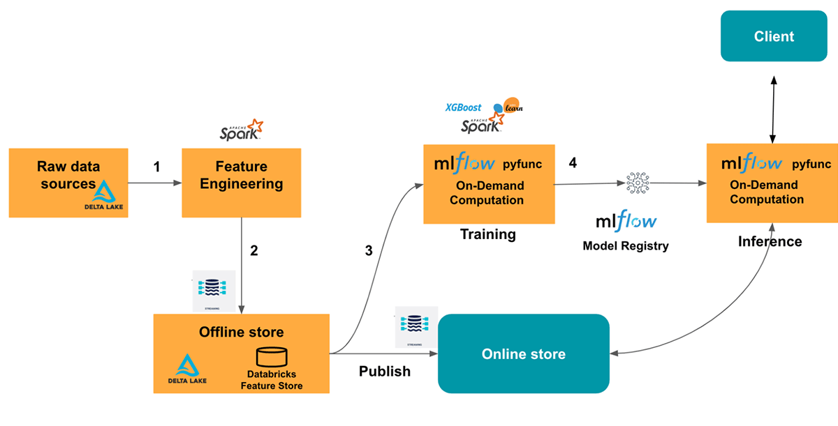
• Batch architecture - for any type of data where an update frequency of hours or days is acceptable, we will use batch computation, using Spark and feature store write_table API, and then publishing the data to the online store. This applies to: Destination location data and Destination popularity data.

fs.write_table(
   name="travel_recommendations.location_features",
   df=destination_location_df)
fs.publish_table("travel_recommendations.location_features",
   destination_location_online_store_spec)

• Streaming architecture - for data where data freshness is within minutes we will use Spark Structured Streaming to write to feature tables in the offline store and publish to the online store. This applies to: Destination availability data. Making the switch from batch to streaming on Databricks is straightforward due to consistent APIs between the two. As demonstrated in the example, the code remains largely unchanged. You only need to use the streaming data source in feature computation and set the "streaming = True" parameter to publish features to online stores.

destination_availability_df = spark.readStream.format("kafka").load()
fs.write_table(
   name="travel_recommendations.availability_features",
   df=destination_availability_df,
   mode="merge")
fs.publish_table("travel_recommendations.availability_features",
   destination_availability_online_store_spec,
   streaming = True)

• On-Demand architecture - for features that are only computable at the time of inference, such as user location, the effective data freshness requirement is "immediate" and we can only compute them on-demand. For those features we will use on-demand architecture. This applies to: user preferences feature - the distance between user location and destination location.

# Wrap the model with on-demand feature computation layer
class OnDemandComputationModelWrapper(mlflow.pyfunc.PythonModel):
   def predict(self, context, model_input):
       new_model_input = self._compute_ondemand_features(model_input)
       return  self.model.predict(new_model_input)
   ...

On-demand Feature Computation Architecture

We want to compute on-demand features with contextual data such as user location. However, computing the on-demand feature in training and serving can result in offline/online skew. To avoid that problem we need to ensure that on-demand feature computation is exactly the same during training and inference. To achieve that we will use an MLflow pyfunc model. Pyfunc model gives us the ability to wrap model prediction/training steps with a custom preprocessing logic. We could reuse the same code for featurization in both model training and prediction. This helps reduce any offline and online skew.

Sharing featurization code between training and inference

In this example we want to train a LightGBM model. However, in order to ensure we have the same feature computation used in Online model serving and Offline model training, we use an MLflow pyfunc wrapper on top of trained model to add custom preprocessing steps. The pyfunc wrapper, adds a on-demand feature computation step as a preprocessor which gets called during training as well as inference time. This allows the on-demand feature computation code to be shared in offline training and online inference, reducing the offline and online skew. Without the common place to share code for on-demand feature transformation, it's likely code to do training will end up using a different implementation than inference resulting in hard to debug model performance problems. Let's look at the code, we are calling the same _compute_ondemand_features in model.fit() and model.predict().

# On-demand feature computation model wrapper
class OnDemandComputationModelWrapper(mlflow.pyfunc.PythonModel):
      
   def fit(self, X_train: pd.DataFrame, y_train: pd.DataFrame):
       new_model_input = self._compute_ondemand_features(X_train)
       self.model = lgb.train(
           lgb.Dataset(new_model_input, label=y_train.values),
           5)
          
   def predict(self, context, model_input):
       new_model_input = self._compute_ondemand_features(model_input)
       return  self.model.predict(new_model_input)

   def _compute_ondemand_features(self, model_input: pd.DataFrame)->pd.DataFrame:
       loc_cols = ["user_longitude","user_latitude","longitude","latitude"]
       model_input["distance"] = model_input[loc_cols].apply(lambda x: my_distance((x[0], x[1]), (x[2], x[3])), axis=1)
       return model_input

Deployment to production

Let's deploy the model to the Databricks Model Serving. Because the Feature Store logged model contains lineage information, the model deployment automatically resolves Online Stores required for feature lookup. Served model automatically looks up the features from just the user_id and destination_id (AWS|Azure) so our application logic can stay simple. Additionally, MLflow pyfunc allows us to make the recommendations more relevant, by computing the on-demand features like distance of the user from destination. We will pass the realtime features such as user_latitude and user_longitude as part of our input request to the model. MLflow model's preprocessor will featurize the input data into distance. This way our model can take context features like current user location into account when predicting the best destination to travel.

Let's make a prediction request. We will generate recommendations for two customers. One is located in New York and has preference for short distance travel based on the history of their bookings (user_id=4), and another is in California and has long distance travel preference (user_id=39). The model generates following recommendations:

{
  "dataframe_records": [
    # Users in New York, see high scores for Florida 
    {"user_id": 4, "booking_date": "2022-12-23", "destination_id": 16, "user_latitude": 40.71277, "user_longitude": -74.005974}, 
    # Users in California, see high scores for Hawaii 
    {"user_id": 39, "booking_date": "2022-12-23", "destination_id": 1, "user_latitude": 37.77493, "user_longitude": -122.41942} 
  ]
}

# Result with predictions greater than 0.2 indicate high likelihood 
# of purchase
{'predictions': [0.4854248407420413, 0.49863922456395]}

We can see that the highest scoring destination for the user in New York is Florida (destination_id=16), whereas for the user in California the recommended destination is Hawaii (destination_id=1). Our model was able to take into account the current location of the users and use it to improve relevance of the recommendations.

Notebook

You can find complete notebook that illustrates the example above here: (AWS|Azure)

Getting Started with your Realtime Feature Computation

Determine for your problem, whether you need realtime feature computation. If yes, figure out what type of data you have, data freshness and latency requirements.

• Map your data to batch, streaming, and on-demand computational architecture based on data freshness requirements.
• Use spark structured streaming to stream the computation to offline store and online store
• Use on-demand computation with MLflow pyfunc
• Use Databricks Serverless realtime inference to perform low-latency predictions on your model

Credits

We would like to express our sincere gratitude to Luis Moros, Amine El Helou, Avesh Singh, Feifei Wang, Yinxi Zhang, Anastasia Prokaieva, Andrea Kress, and Debu Sinha for their invaluable contributions to the ideation and development of the example notebook, dataset and diagrams. Their expertise and creativity have been instrumental in bringing this project to fruition.