Fleet optimization with CARTO & Databricks

Effective delivery has become increasingly important for businesses in recent years, particularly for logistics companies and those in the consumer packaged goods (CPG) industry that have their own distribution networks.

A big challenge for these companies is optimizing transportation routes to minimize costs while ensuring timely delivery. This involves considering factors such as distance, traffic, road conditions and the type of transportation used (e.g., truck, rail, air). Additionally, CPG and logistics companies must consider the environmental impact of their transportation choices and aim to reduce their carbon footprint. With increases in fuel prices and intensifying competition, it is crucial for these organizations to develop clear plans to become more sustainable, address transportation issues, and lower overall delivery costs.

Routing software is a key tool that helps companies to tackle these challenges by:

• Planning better routes, decreasing overall fuel consumption and maintenance expenses
• Optimizing delivery times to customers
• Getting clear, up-to-date insights on the delivery network, including a graphical representation of routes in a geographical context
• Using quantitative analysis of routes through a set of Key Performance Indicators
• Taking advantage of additional data sources such as road traffic and weather data as part of a constraint-based optimization approach

Read on to find out how Databricks and our partner CARTO can help you optimize your logistics strategy, making your delivery processes and routes more efficient and cost-effective.

The Vehicle Routing Problem

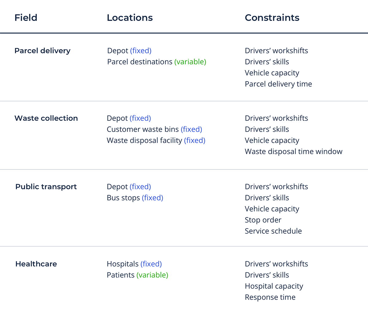
The Vehicle Routing Problem, or VRP, is a class of optimization problems through which we try to find the most optimal routes for a fleet of vehicles to visit a set of locations while satisfying different constraints. From an analytical perspective, when dealing with VRP, we have to consider many varied constraints as outlined in the following table:

VRP is a generalization of a simpler use case, the traveling salesperson problem (TSP):

If we had a number of cities to visit, what would be the shortest route to pass exactly one time by each city and come back to the original city?

In the TSP, we have a single vehicle that has to visit all cities in the shortest possible route with the only constraint being not visiting the same city twice. The main difference between TSP and VRP, is that in VRP we consider a fleet, instead of a single vehicle, and have to factor in a series of additional constraints.

VRP = Locations + Vehicle fleet + Constraints + Magnitudes to optimize

VRP problems are varied in scope and complexity, and cover many scenarios outlined below:

• Vehicles can take more than one route -> VRP with Multiple Trips (VRPMT)
• Vehicles don't need to return to their original location -> Open VRP (OVRP)
• Vehicles can start and end in different depots -> Multi Depot VRP (MDVRP)
• Vehicles can carry goods up to a certain capacity -> Capacitated VRP (CVRP)
• Locations can only be visited within specific time windows -> VRP with Time Windows (VRPTW)

This is just a selection of the options available. And to further complicate matters, new VRPs can be defined using a combination of all of the above.

In their general form, VRP problems are challenging to solve! They belong to a category known as NP-hard problems. The time required to solve these problems increases rapidly with the size of their input data.

A naive approach to solving a VRP would be:

1- Compute all the possible solutions as combinations of vehicles and locations they visit
2- Discard the solutions that do not satisfy the constraints
3- Compute some sort of score to measure how good each solution is
4- Select the solution with best score

As the number of vehicles and locations to visit increases, the number of combinations of routes grows factorially. For example, let's suppose we have a computer able to perform 1.000.000.000 operations in a second. Let's see how much time would take to solve different sizes of VRP's:

It is not rare to find real cases in which the number of locations to visit is several thousand. So it is clear that to find solutions for VRPs, we have to use methods that provide solutions that may not necessarily be the best, but that can be computed in a shorter amount of time. Even if we apply techniques to simplify/partition our problem, there is still the need for scaling up the processing. Databricks Lakehouse platform naturally fits the variety of needs that a complex problem like VRP poses.

Several libraries implement VRP algorithms and allow us to develop software to optimize routes for vehicle fleets. But building these solutions from scratch is not an easy task. Even making use of these available libraries involves the following considerations:

• Fully understanding the routing library requires a steep learning curve. Our solution provides an abstraction layer and simplifies the end to end journey from the problem statement to VRP solution.
• VRP is resource-hungry and careful management of computational resources is required to deploy an enterprise scale application:
  • Scaling and load balancing. Databricks Lakehouse platform can be a powerful ally in VRP, where a high computing power is required, but only during certain time slots.
  • Resiliency. Databricks being a PaaS cloud offering abstracts the need to handle resiliency manually by the end users, the platform takes care of ensuring resources are available and that VRP can be run on demand.
• Additional aspects apart from the VRP must also be taken into account:
  • Graphical representation of data in a geographical context. Integration between CARTO and Databricks provides a great mix between scalable compute and interactive geospatial UI.
  • Additional insights such as charts or metrics that provide key performance indicators about the performance of the solution. MLFlow provides a set of capabilities to collate different aspects of VRP solutions and produce a comprehensive audit trail.

Introducing Carto's Fleet Optimization Solution using Databricks

To address this complex spatial problem, CARTO provides a fleet optimization toolkit that allows developers to take full advantage of the powerful and elastic computing resources of Databricks to design routing applications that help companies to be more efficient, competitive and environment-friendly.

CARTO's routing solution provides several ready-made components. Different elements of this framework can be defined, allowing users to set the specific details of the routing problem.

The following diagram depicts the process of solving a routing problem using the CARTO routing module on Databricks.

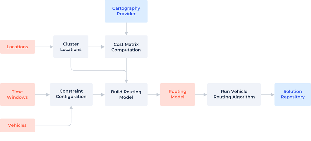
These are the main components of the solution:

• Vehicle Routing Algorithm. Computes valid solutions for the VRP it is fed as its input.
• Routing Model. Contains the problem setting, including stops, constraints, route cost matrix and everything else the routing algorithm needs as input
• Cartography Provider. Provides the traffic maps that will be used to determine the travel path between every pair of stops in the problem.
• Location Clustering. Arranges locations that are near enough into groups called "stops", in order to reduce the size of the problem. Different clustering algorithms can be defined.
• Constraint Configuration. Creates constraints from Time Windows and drivers, in order to add them to the routing model.
• Solution Repository. After the routing algorithm has ended successfully and a solution has been computed, it can be stored in a Solution Repository like Delta Lake.

Here is a sample code that could be used to design an applications with these components:

1. First code example. Preparing network data.

   """
      Download geographic data from Open Street Map and process it to
      obtain the network to compute distance matrices.
      This code could be run on a periodic basis, in order to have
      network data up to date (daily, weekly, monthly), but as we have it
      stored on DBFS, it can be reused as many times as we need
      without needing to re-run the script.
   """
   
   from carto_vrp.osm import OSMDataset
   from carto_vrp.network import Network
   
   # Select the geographical area of the data to be downloaded
   osm_pbf_url = 'http://download.geofabrik.de/europe/france/ile-de-france-latest.osm.pbf'
   
   # Download dataset from OSM as network provider
   osmd = OSMDataset(osm_pbf_url)
   
   # We will store network data in DBFS
   output_folder = '/dbfs/FileStore/routing_optimization_data/paris'
   
   # Instantiate network builder
   ntwk = Network(osmd)
   ntwk.build(output_folder)
   
   # from this point, network data is available at the DBFS output folder

2. Second code example: solving a fleet optimization problem:

   """
      Load a VRP dataset and network data and generate a solution.
      The VRP dataset includes jobs (i.e. deliveries), vehicles and a depot.
      The network data provides all the information needed to compute travel costs
      between different locations.
      VRP dataset and solution are stored in Delta Lake.
   """
   
   from carto_vrp.problem import VehicleCostMatrix
   from carto_vrp.repository import VRPRepositoryDelta, VRPSolutionRepositoryDelta
   from carto_vrp.routing_algorithms import VehicleRoutingAlgorithm
   from carto_vrp.routing_engine import RoutingEngine
   from carto_vrp.vehicle import Vehicle
   import mlflow
   
   
   # Loading dataset from Delta Lake tables from Delta Lake.
   # We provide a spark session and three tables from which recover
   # Jobs, Vehicles, Metadata, including depot location
   vrp_repository = VRPRepositoryDelta(spark, 'carto_data.vrp_jobs_paris',
                                     'carto_data.vrp_vehicles_paris',
                                     'carto_data.vrp_metadata_paris')
   vrp_dataset = vrp_repository.load()
   
   
   # Instantiate a RoutingEngine, the interface to network data
   network_data = '/dbfs/FileStore/routing_optimization_data/paris/paris-latest.osrm'
   routing = RoutingEngine({Vehicle.DEFAULT_VEHICLE_TYPE: network_data})
   
   # Compute a cost matrix based on network data provided
   cost_matrix = VehicleCostMatrix(routing, vrp_dataset)
   
   # Instantiate the algorithm to find the solution to the VRP statement
   algorithm = VehicleRoutingAlgorithm(vrp_dataset, cost_matrix)
   solution = algorithm.search_solutions()
   
   # this provides a short digest of the VRP solution obtained
   print(solution)
   # use mlflow to store metadata about the VRP solution
   with mlflow.start_run():
   	mlflow.log_param("municipality", "Paris")
   	mlflow.log_param("network_data_location", network_data.dataset_name)
   	mlflow.set_tag("solution_digest", solution.summary)
   
   # Now, we can store the solution in Delta Lake, from which
   # we can use CARTO to display it graphically
   solution_repo = VRPSolutionRepositoryDelta(routing,
   'carto_data.vrp_nodes_paris',
   'carto_data.vrp_edges_paris')
   solution_repo.save(solution)

In the examples above we have demonstrated how effortless it is to build the code for a VRP solution using CARTO's routing solution. Through seamless integration with Databricks Lakehouse platform these solutions can easily be scaled up and we can run many VRP problems in parallel using Databricks scalable compute, at the same time we can easily keep track of different subproblems using MLFlow to collate the metadata about different runs.

Example use case: a CPG company delivering to various retailers

To illustrate the importance of effective delivery and logistics for CPG companies, let's consider a practical use case of a CPG company with its own distribution network. The CPG company places a number of products to be delivered to their various retailers on a given due date, with most of these products having a specific time window for delivery.

To optimize its distribution network, the company estimates the number of vehicles required to deliver all the products and aims to optimize their transportation routes to minimize costs while ensuring timely delivery.

The solution to the VRP has to take into consideration many additional aspects such as:

Our fleet is composed of a number of vehicles and their drivers. They must go from the depot to the retailers, thus describing routes. We've got some things we need to optimize: we want to deliver as many products as possible, in as little time as possible, and with as few vehicles as possible. We've also got a few constraints we need to work with, like the delivery time windows, driver work shifts, and vehicle capacity.

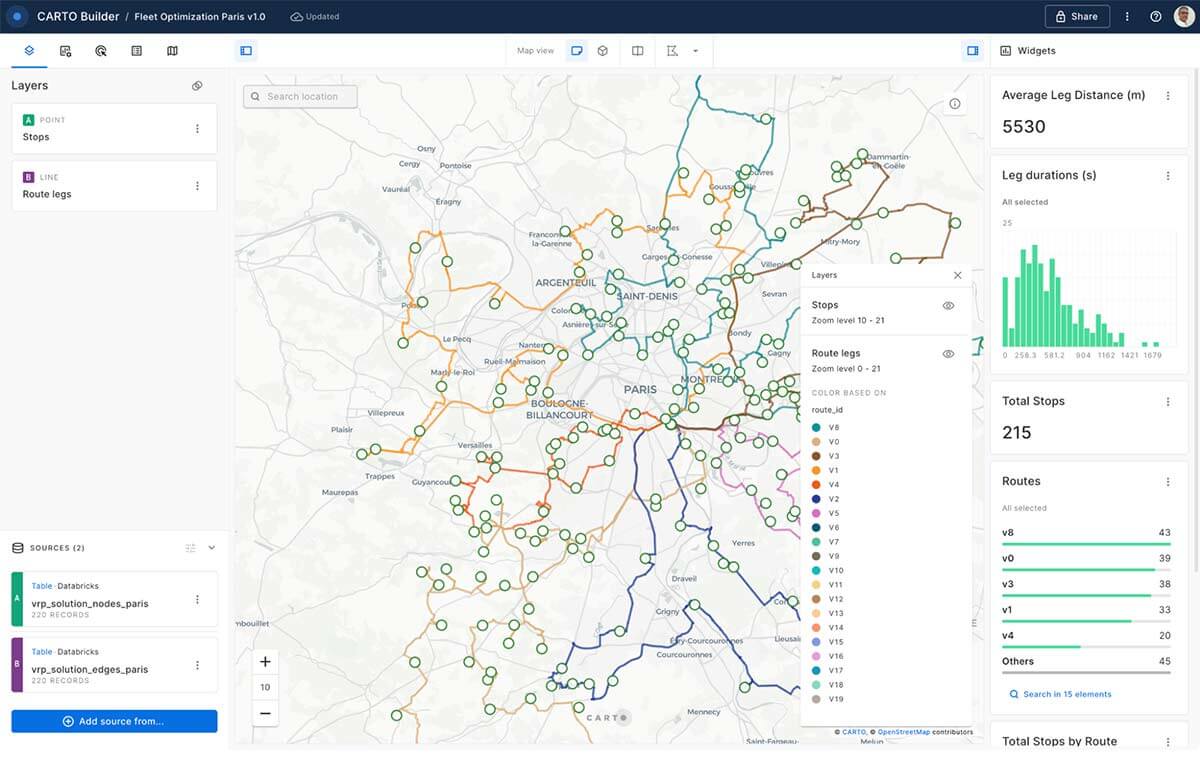
Every day, in the early morning, we run the fleet optimization process to solve the daily VRP. As a result, we obtain a set of routes that our drivers should take, with a nice map to help visualize them. We also get a list of the stops we must make and the products we will deliver at each one. Each route is assigned to a specific vehicle, and we can track a few KPIs to help us see how we're doing. For example, we can see how many stops we made in total and the average distance each route leg covers. Additionally, we can view a histogram graph to represent the route leg durations.

Good route optimization can provide the company with a competitive advantage. By optimizing their distribution network, they can offer faster, more cost-effective and more reliable delivery than their competitors, which can help them increase market share.

If you want to see how the CARTO & Databricks fleet optimization solution can be applied to your use case, don't hesitate to reach out!