How Databricks Powers Stantec's Flood Predictor Engine
by Assaad Mrad, Jared Van Blitterswyk, Ricardo Piscitelli and Liliana Tang
This is a collaborative post between Stantec and Databricks. We thank ML Operations Lead Assaad Mrad, Ph.D. and Data Scientist Jared Van Blitterswyk, Ph.D. of Stantec for their contributions.
At Stantec, we set out to develop the first ever rapid flood estimation product. Flood Predictor is built upon a ML algorithm trained on high-quality features. These features are a product of a feature engineering process that ingests data from a variety of open datasets, performs a series of geospatial computations, and publishes the resulting features to a feature store (Figure 1). Maintaining the reliability of the feature engineering pipeline and the observability of source, intermediate, and resultant datasets ensure our product can bring value to communities, disaster management professionals, and governments. In this blog post, we’ll explain some of the challenges we have encountered in implementing production grade geospatial feature engineering pipelines and how the Databricks suite of solutions have enabled our small team to deploy production workloads.
![Figure 1: Data flow and machine learning overview for flood predictor from raw data retrieval to flood inundation maps. Re-used from [2211.00636] Pi theorem formulation of flood mapping (arxiv.org).](https://www.databricks.com/sites/default/files/inline-images/db-405-blog-img-1.png)
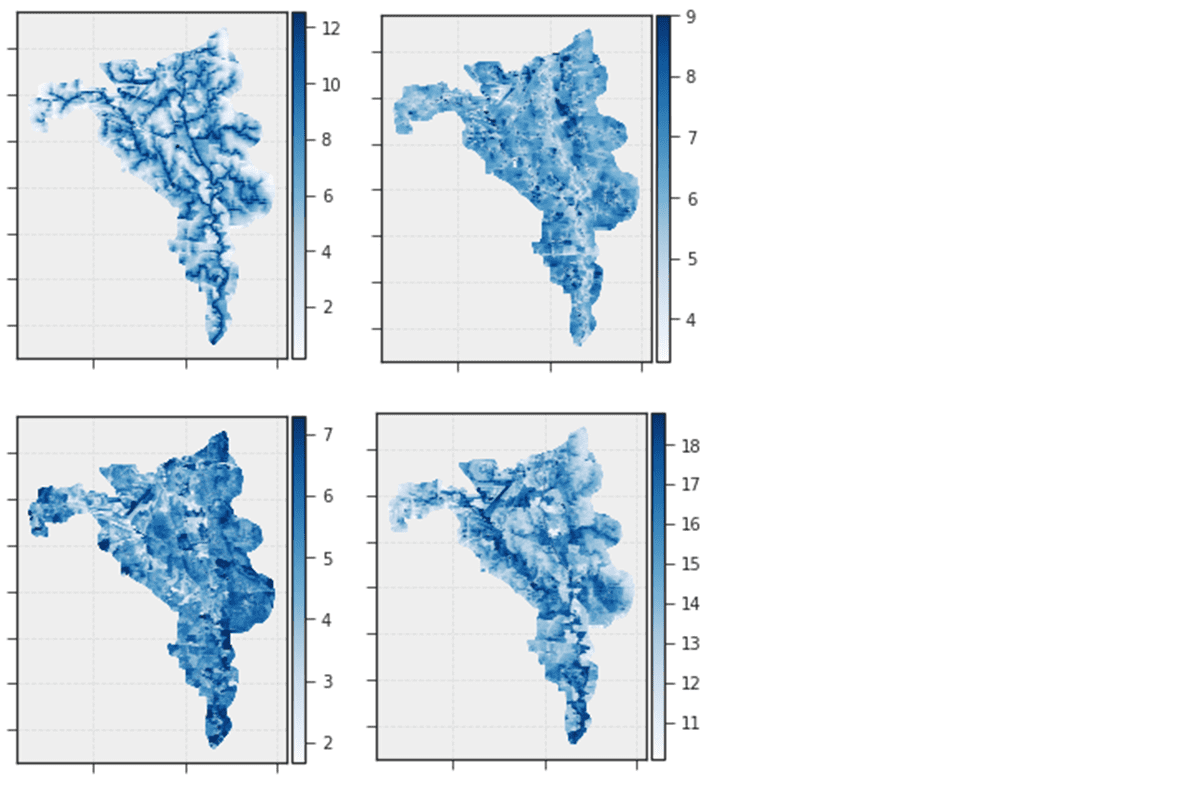
The abundance of remote sensing data provides the potential of rapid, accurate, and data-driven flood prediction and mapping. Flood prediction is not straightforward, however, as each landscape has unique topography (e.g., slope), land use (e.g., paved residential), and land cover (e.g., vegetation cover and soil type). A successful model would be explainable (engineering requirement) and general: able to perform well over a wide range of geographical regions. Our initial approach was to use direct derivatives of the raw data (Figure 2) with minimal processing like normalization and encoding. However, we found that the generalization of the predictions was not sufficient, model training was computationally expensive and the model was not explainable. To address these issues, we leveraged Buckingham Pi theorem to derive a set of dimensionless features (Figure 3); i.e. features that do not depend on absolute quantities but on the ratio of combinations of hydrologic and topographic variables. Not only did this reduce the dimensionality of the feature space, but the new features capture the similarity in the flooding process across a wide range of topographies and climate regions.
By combining these features with logistic regression, or tree-based machine learning models we are able to produce flood risk probability maps, compared to more robust and complex models. The combination of feature engineering and ML allows us to expand flood prediction in new areas where flood modeling is scarce or not available and provides the basis of rapid estimation of flood risk on a large scale. However, modeling and feature engineering with large geospatial datasets is a complicated problem that can be computationally expensive. Many of these challenges have been simplified and become less costly by leveraging capabilities and compute resources within databricks.
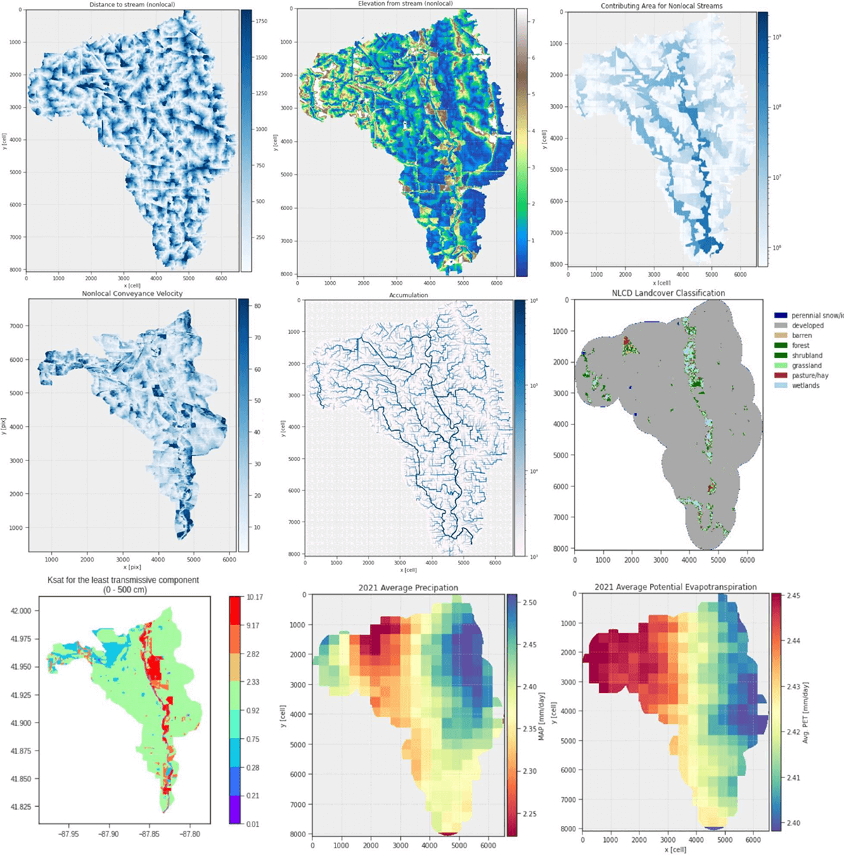
Figure 2: Illustrative maps of the dimensional features first used to build the initial model for the 071200040506 HUC12 (12-digit hydrologic unit code) from the categorization used by the United States Geological Survey (USGS Water Resources: About USGS Water Resources).
Each geographical region consists of tens of millions of data points, with data compiled from several different data sources. Computing the dimensionless features requires a diverse set of capabilities (e.g., geospatial), substantial compute power, and a modular design where each “module” or job performs a constrained set of operations to an input with a specific schema. The substantial compute power required meant that we gravitated toward solutions that were cost-effective yet suitable for large amounts of data and Databricks Delta Live Tables (DLT) was the answer. DLT brings highly configurable compute with advanced capabilities such as autoscaling and auto-shutdown to reduce costs.
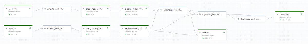
During the conceptual development of Flood Predictor we placed emphasis on the ability to quickly iterate on data processing feature creation, and less priority on maintainability and scalability. The result was a monolithic feature engineering code, where dozens of table transformations were performed within a few python scripts and jupyter notebooks, it was hard to debug the pipeline and monitor the computation. The push to productionizing Flood Predictor made it necessary to address these limitations. The automation of our feature engineering pipeline with DLT enabled us to enforce and monitor data quality expectations in real-time. An additional advantage is that DLT breaks the pipeline apart into the views and tables on a visually pleasing diagram (Figure 4). Additionally, we set up data quality expectations to catch bugs in our feature processing.
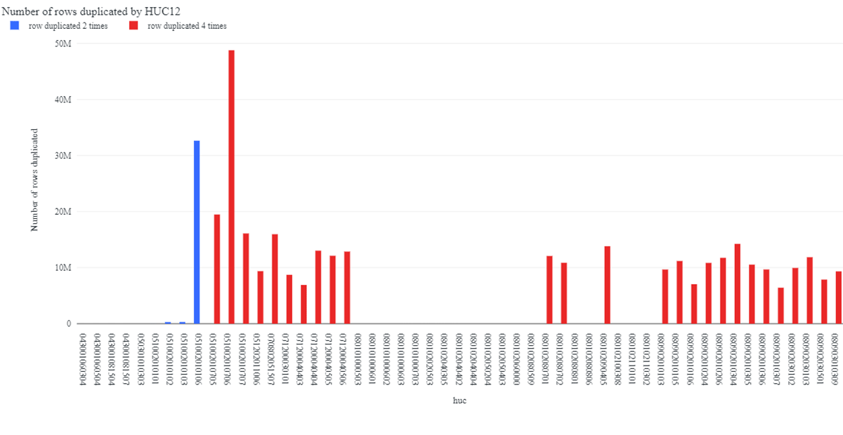
The high-level pipeline visualization and pipeline expectations make maintenance and diagnostics simpler: we are able to pinpoint failure points, go straight to the offending code and fix it, and load and validate intermediate data frames. For example, we were able to discover that our transformations were leading to pixels or data points being duplicated up to four times in the final feature set (Figure 5). This was more easily detected after setting an “expect or fail” condition on row duplication. The chart in Figure 5 automatically updates at each pipeline run as a dashboard in the Databricks SQL workspace. Within a few hours we were able to identify that the culprit was an edge case where data points on the edge of the maps were not properly geolocated.
We now return to an earlier point: we need our flood prediction system to be as widely applicable (general) as possible. How do we quantify the ability of a trained Machine Learning model to to generalize beyond regions within the training datasets? The geospatial dependency of points in our datasets requires care when partitioning data into training and test sets. For this we use a variant of the cross-validation technique called spatial cross validation (e.g.: https://www.nature.com/articles/s41467-020-18321-y) to compute evaluation metrics. The overarching idea of spatial cross-validation is to split the features and labels into a number of folds based on geographical location. Then, the model is trained successively on all but one fold, leaving one fold out at each step. The evaluation metric (e.g., root mean squared error) is computed for each step and a distribution is obtained. We had 10 subwatersheds with labels to train on so we applied a 10-fold spatial cross-validation where each fold is a subwatershed. Spatial cross-validation is a pessimistic metric because it may leave out a fold with features that are not representative of the set of training folds, but this is exactly the high-standard we want our dimensionless features and model to achieve.
With our features and evaluation process in place the next step is training the model. Fortunately, training a statistical model on a large data set is straightforward in Databricks. Ten subwatersheds contain on the order of 100 million pixels, so the full training set does not fit into the memory of most compute nodes. We experimented with different types of models and hyperparameters on a subset of the full data on an interactive Databricks cluster. Once we settled on a given algorithm and parameter grid, we then defined a training job to take advantage of the lower cost for job clusters. We use PySpark’s MLLib library to train a scalable Gradient-Boosted Tree classifier for Flood Predictor and let MLflow monitor and track the training job. Choosing the right metric to evaluate a model for flooding is important; for most events, the frequency of ‘dry’ pixels is much higher than that of flooded pixels (on the order of 10 to 1). We chose to compute the harmonic mean of precision and recall (F1 score) about the flood pixels as a measure of model performance. This choice was made because of the large imbalance in our target labels and classification threshold invariance is not desirable for our problem.
Unlike other forms of data, a user requests geospatial data by delineating a bounding box, a shape file, or by referencing geographical entities like cities. A typical request for Flood Predictor output specifies a bounding box in decimal degree coordinates, and a precipitation depth such as 3.4 inches. The server side application ingests those inputs, in a JSON format, and queries the feature store for the pixel features within the requested bounding box. As is typical for geospatial data services, the returned output is not at the level of a single pixel, but pre-defined tiles containing a given number of pixels. In Flood Predictor’s case, each tile contains 256x256 pixels. The advantage of this approach is proactively limiting the data volume served by the API to maintain satisfactory response times and not overload the database nodes. To achieve this design, we tag each pixel in the database with a tile ID that specifies the tile it belongs to. So, after the user query is ingested, the server side application finds the tiles that intersect the requested bounding box and predicts flooding for these areas. With this design, Flood Predictor can return high-quality flood predictions for dozens of square miles at 3-10 meters of resolution within only minutes.
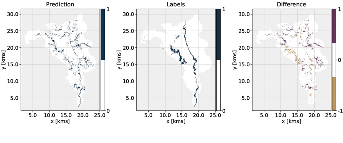
Figure 6: Flood predictor output compared to the label from 2D hydraulic and hydrologic modeling for the 071200040506 HUC12 and a 10-year storm event. These are categorical maps where “1” denotes flooded areas. The resolution of the map is 3 meters and downsampled by a factor of 100 for visualization purposes.
Flooding is fundamentally a geospatial random process that is constrained by spatial patterns of topography and land cover and affects a substantially large number of communities and assets. This is why flood prediction has been the subject of numerous physical and statistical models of varying quality but there exists, to our knowledge, no comparable product to Flood Predictor. Databricks has been a decisive factor for Flood Predictors success: it was by far the most cost-effective way for a small team to quickly develop a proof-of-concept prediction tool with available datasets, as well as implement production-grade jobs and pipeline.
Backed by Databricks’ end-to-end machine learning operations, Stantec’s enterprise-grade Flood Predictor helps you get ahead of the next flooding events and save lives through well-designed predictive analytics. Check it out on the Santec website: Flood Predictor (stantec.com) and on the Microsoft Azure marketplace.
Get the latest posts in your inbox
Subscribe to our blog and get the latest posts delivered to your inbox.