Managing Recalls with Barcode Traceability in the data lakehouse

Recent data show that the number of recall campaigns caused by product deficiencies keeps increasing, while each known recorded case is a multi-million Dollar damage on average. Additional reputational- as well as business continuity- risks demonstrate the downside potential of each recall being "a bottomless pit". Product recalls are not only a matter of traditional manufacturing companies of all sizes, they are relevant for every company that produces a product, e.g. pharmaceutical companies. In this article, we argue why a central data lakehouse on top of multiple production plants dramatically helps reduce affected damage by shortening problem-solving cycle times. We further present a solution accelerator that gives precise examples for traversing process graphs to detect operational deficiencies.

Challenges and Chances of Data Analysis for Effective Management of Recalls

A Note on Recalls

In a situation in which a manufacturer produces and ships products to a customer, a product recall is a request from either party to return a product after the discovery of severe quality problems. For example, Mercedes recalled approximately 144,000 vehicles because of a defect in the fuel pump (see here) and BSH recalled 170,000 gas stoves that could explode (see here). Recalls can affect a long range of the value chain, including the product's manufacturer, its customers as well as its suppliers. Potential damages are:

• Nonconformance costs (NCC): NCCs are the direct costs resulting from quality issues. Examples are scrap costs, downtime costs, warranty claims, or recall costs.
• Reputational risks: As a result of a quality issue, the manufacturer can be downgraded in the customer's quality perception. This may result in lost sales.
• Business continuity risks: In the problem-solving phase, the manufacturer might decide to stop producing and shipping products to their customers to prevent further damage. Note that this is not completely orthogonal to NCC.

According to Statista, recalls in a manufacturing-intensive economy like Germany increased in recent years. Furthermore, a study by Allianz (see here) shows that a "major" recall leads to damage of 10.5 Million Euros. However, domino effects may make this damage much larger. Examples span a wide range of affected industries, like Automotive, Food and Beverage of IT / Electronics.

Managing recalls can be twofold.

• If the product is already shipped to the customer, the manufacturer of the affected product must eliminate and explain the operational problem as fast as possible to ensure the continuity of their operations. Furthermore, a customer often recalls a complete time range even though only a couple of barcodes are affected. Explaining the issue with data and thereby proving which barcodes are affected can dramatically reduce the damage.
• In case of an issue in the production process or a known defect with one of the supplier's raw materials the manufacturer of the affected product must identify affected production steps and barcodes as fast as possible and eliminate the operational problem.

Both cases require traversing the manufacturing value chain on a barcode level either back- or forwards and explaining the issue with operational data. Data is the key to effective and fast recall management!

The Problem With Finding and Analyzing the "Right" Data

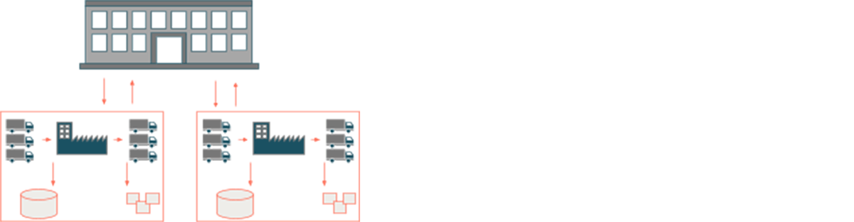
The data landscape in an organizational structure with multiple plants that are managed by a central department can be problematic. Let's assume that each plant is supplied with raw materials (indicated with trucks coming in) before a product is assembled and the finished product is shipped to the customer (indicated with trucks going out). Two operational systems matter. On the one hand, there is a Manufacturing Execution System (MES) that controls the process of manufacturing goods from raw materials to finished products and on the other hand there is a planning system (often SAP) that controls the logistics steps of the finished product. Two different systems introduce challenges when traversing the value chain within one plant. Multiple plants multiply the magnitude of this problem by the number of plants. More precisely:

• No central view - Plant-local MES build data silos the central department must traverse products of each plant independently, instead of drilling down from a central level to the plant level in an automatic fashion.
• Missing data literacy - There is a small number of plant-local experts to analyze the data. The central department is often alien to the specifics of each plant and finds it difficult to understand and analyze the plant's operational data.
• Missing scalability - The aforementioned operational systems are often subject to on-prem databases as the minimum level of trust to migrate to the cloud (given known outages in some regions) is not given. On the other hand, the storage and computational resources of traditional on-premises systems are not independently scaleable, which hinders the onboarding of data-centric use cases.
• Blind spot - On-prem systems have problems with unstructured and streaming data, introducing an operational blind spot.

The Lakehouse On Top of Multiple Plants

To mitigate the aforementioned challenges, many manufacturers use Databricks to build a data lakehouse on top of multiple production plants. The "Lakehouse on top of multiple production plants" is a standardized "copy" of the plant-local operational systems. Files are stored in the Delta Lake format, an open source storage format that consists of Parquet files with a layer of metadata that ensures cost-efficiency, scalability, and highly performant data queries and transformations for production workloads. Data governance features like data access controls and audibility are easily applicable with the help of the Unity Catalog. This architecture represents a unified platform for data-intensive manufacturing use cases, including data warehousing, dashboarding, machine learning, data science or data engineering. For a manufacturer, this offers significant benefits:

• It provides a central view by collecting production data of all plants. A drill-down from the central to the plant level is easily possible in an automated fashion.
• The standardized data copy reduces the dependency on specific resources within one plant.
• The cloud itself provides independent scalability of storage and computational resources which dramatically facilitates onboarding of data-intensive use cases.
• All data of all formats can be stored in a cost-efficient way on cloud object storage.
• Streaming events can be ingested in the data lakehouse with low latency

While this article focuses on recalls, the advantages of the lakehouse on top of multiple production plants are much larger. Examples include multi-plant overall equipment efficiency, active production quality monitoring, or product delivery tracking. In this article, we focus on combining the right data at the right time for each manufactured barcode, which is the central methodology for structured problem solving, i.e. barcode traceability.

Three Examples of Barcode Traceability and a Simple Data Model to Tackle Them

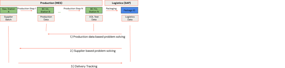
The production process consists of stations, in which products are being processed. The products are represented by barcodes. Each barcode is unique in one station within one plant. The manufacturer's production process starts with raw materials that come from a supplier. Barcodes may change along the production process, for example as a result of an assembly step. At each station, further data is generated, e.g. supplier batches, machine data, or test data. The above process is simplified, as it may contain splits or merges. Logistics steps can be seen in exactly this way, just that the operational steps would be specific to logistics, e.g. packaging, and a package ID would enter the process. The sequence of production and logistics steps form a manufacturing process graph. In this setting, we consider three examples:

1. Production data-based problem solving: The manufacturer produces and ships barcodes to a customer. The customer finds that a considerably large number of products have an issue and recalls a complete production time range. The manufacturer must eliminate the production deficiency and explain ideally with data that a limited number of barcodes are actually affected. For this purpose, the manufacturer takes a limited number of barcodes that have a known issue and analyzes relevant production data in its production process. The relevant data is identified by traversing the operational production process backward. This is backward traceability.
2. Supplier-based problem solving: This is similar to the first example, just that the backward traceability is performed to the very beginning of the production process where the raw materials enter production. If the analysis reveals that all issues can be traced back to one and the same supplier batch, this is suspicious and can lead to further supplier quality analysis.
3. Delivery tracking: A supplier ships raw materials that enter a manufacturer's production process before the resulting finished products are shipped to the customers. The supplier finds that a couple of barcodes do not meet the desired specifications. Unluckily, the affected raw material is already assembled in the manufacturer's products. The manufacturer must identify the affected barcodes and production steps as soon as possible. The relevant barcodes are identified by traversing the operational production process forward. This is forward traceability.

Luckily, the operational production process generates data. We can model these data in various ways. This article demonstrates modeling the data with the help of a very simple table which is able to solve the aforementioned three example use cases.

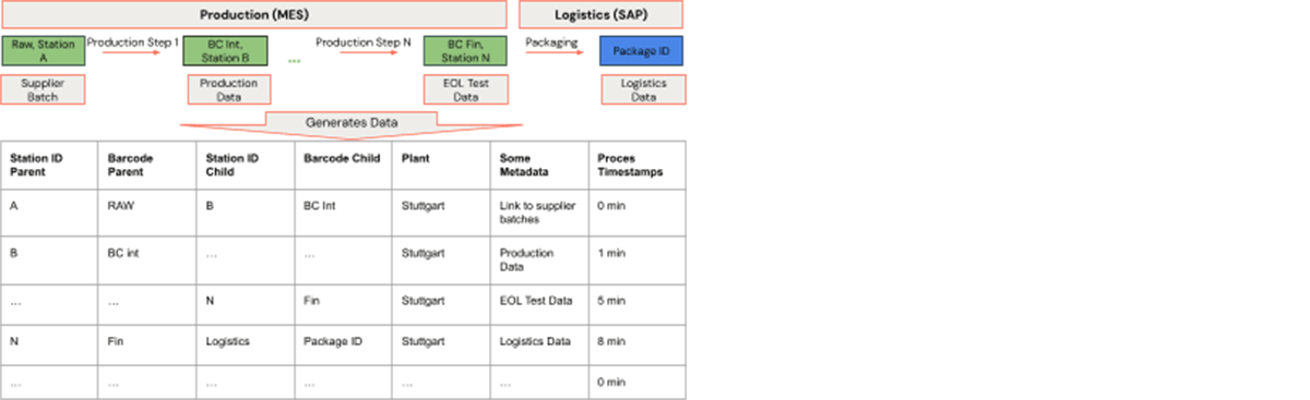
In each process step, the combination of station ID, barcode, and plant forms a unique parent, which is assembled into another combination of these three items. The process has time stamps and other production data, e.g. press fit curves, can be linked. In graph terminology, each row is an edge. The combination of barcode, station ID, and plant form a vertex. All vertices can easily be created for the set of edges. This vertex and edge data form a data representation of the manufacturing process graph. By this means, barcode traceability is a matter of finding neighborhoods of specific vertices in a graph.

The Barcode Traceability Solution Accelerator

The Databricks Solution Accelerators are purpose-built guides tailored to accelerate customers' use case development. They consist of fully functional notebooks and best practices with a solution and industry-specific focus.

In this article, we briefly present a solution accelerator for barcode traceability. Note that many more explanations and code can be found in the Git Repo. Here, we walk through the basic steps, i.e. the code snippets related to each of the three examples described above. In each example, we present a different methodology for traversing the graph. This is not necessary but demonstrates different methods for traversing a graph. A discussion about the chances and limitations of each methodology is outlined in the notebooks of the solution accelerator.

Note that the solution accelerator is based on a real production example. In this article, we abstract away from the specific production steps and products and instead focus on the code and methodology that can be applied to tackle barcode traceability.

Creating the Manufacturing Process Graph

The process steps are as follows

display(edge_df.select("src","dst","Link_to_data","
Start_Time", "End_Time"))

The columns "src" and "dst" are the parent and child for the graph. They are made of a string concatenation of the barcode, the station id, and the plant. Other data are linked in a column. The process start and end times are recorded as a timestamp. The graph frame can then easily be created.

g = GraphFrame(vertices_df, edge_df)

Example 1: Production Data-Based Problem Solving

This example has a set of barcodes coming from the customer as input and we would like to trace back to a specific station, i.e. the turning station. We will apply Motif Finding to do this. First, we derive a search pattern from a couple of barcodes using Breadth-first search.

example_path = g_reverted.bfs(
 fromExpr = "id = '" + start_search_nodes.collect()[0][0] + "'",
 toExpr = "SID = 'Turning_Blank_Station'",
 maxPathLength = 10)

The result can easily be transformed to a valid search pattern which is an abstraction of the specific subgraph we search for and described by vertices that are connected by edges.

'(from)-[e0]->(v1);(v1)-[e1]->(v2);(v2)-[e2]-
>(v3);(v3)-[e3]->(v4);(v4)-[e4]->(v5);(v5)-[e5]-
>(to)'

The next step is to derive a filter expression. This is straightforward, given that the customer only reported on a couple of barcodes for which the issue was observed.

'to.id in ('MW4EE3C/At_Customer/1',...)'

All suspicious production chains can then be found using

chain = g.find(motif_search_expression).filter(in_expression)

Selecting relevant parts of this output yields a table with all suspicious barcodes at the turning station for every suspicious barcode that the customer reported, as well as the start and end times of the turning process. As the turning station records an endless time series, the timestamps can be used to derive the suspicious parts of the series and problem-solving boils down to a visual inspection of these series.

Example 2: Supplier-Based Problem Solving

This example is similar to the first example. The difference is that we will trace back all the way to the supplier. We could apply the Motif Finding methodology again. To demonstrate different methodologies we apply parallelizing single-threaded Python code with Pandas UDFs. If we manage to decompose the graph into components that are connected within but not across, it suffices to perform traceability within each component independently. Having found all the components we first subset to the relevant components which massively reduces the graph size. In the next step, we apply a single-threaded Python function to do traceability within each component and parallelize using Pandas UDF's.

We first find all connected components.

connected_components_df = g.connectedComponents()

Subsetting to relevant components is a matter of an inner join with the table that lists all suspicious barcodes row-wise.

relevant_components = (connected_components_df.
                     join(start_search_nodes, on = "id", how="inner").
                     select("id", "component").
                     withColumnRenamed("id",
"search_id_in_this_component").
                      distinct()
)

Say, we have a Python function that does the backwards traceability in each component

def ego_graph_on_component(pdf: pd.DataFrame) -> pd.DataFrame:
	...
	return res

Applying the Pandas UDF can be done with

backwards_traceability_df = (
 relevnat_edges
   .groupBy("component")
   .applyInPandas(ego_graph_on_component, output_schema)
)

The result is a table with all suspicious barcodes at the supplier and the respective batches which is then used for further problem-solving.

Example 3: Delivery Tracking

Delivery tracking is tracing the value chain forwards. The supplier at the very beginning of the value chain reports on a couple of suspicious barcodes and the manufacturer has most likely already assembled the raw material in its products. This use case is about identifying the furthermost barcodes in the manufacturer's value chain. We could solve this use case with Motif Finding or with the Pandas UDFs and Python functions as outlined in the two previous subsections. In the Solution Accelerator, we apply the methodology of Message passing via AggregateMessages. It is a primer to send messages between vertices, and aggregate messages for each vertex. We first define the message to be sent between vertices.

msgToDst = AM.edge["aggregated_parents"]

By iteratively sending and aggregating messages along the vertices we can traverse the complete graph.

agg = g_for_loop.aggregateMessages(
 f.collect_set(AM.msg).alias("aggregated_parents"),
 sendToSrc=None,
 sendToDst=msgToDst
)

This easily yields a table with all relevant barcodes for each raw material.

Get Started with Barcode Traceability

Recent data show that the number of recalls increased, while each known recorded case is a multi-million damage on average. This confirms the demand for managing recalls in the most effective way. Different plants with different operational systems introduce data silos that hinder barcode traceability and therefore an effective analysis. A central data lakehouse on top of multiple plants opens the door to a centralized analysis of product deficiencies. Try our solution accelerator to build barcode traceability at your organization, and improve the effectiveness of your data analysis for product deficiencies by dramatically reducing problem-solving cycle times.

Try our solution accelerator to build barcode traceability at your organization, and improve the effectiveness of your data analysis for product deficiencies by dramatically reducing problem-solving cycle times.