Introducing Window Functions in Spark SQL

Get an early preview of O'Reilly's new ebook for the step-by-step guidance you need to start using Delta Lake.

In this blog post, we introduce the new window function feature that was added in Apache Spark. Window functions allow users of Spark SQL to calculate results such as the rank of a given row or a moving average over a range of input rows. They significantly improve the expressiveness of Spark’s SQL and DataFrame APIs. This blog will first introduce the concept of window functions and then discuss how to use them with Spark SQL and Spark’s DataFrame API.

What are Window Functions?

Before 1.4, there were two kinds of functions supported by Spark SQL that could be used to calculate a single return value. Built-in functions or UDFs, such as substr or round, take values from a single row as input, and they generate a single return value for every input row. Aggregate functions, such as SUM or MAX, operate on a group of rows and calculate a single return value for every group.

While these are both very useful in practice, there is still a wide range of operations that cannot be expressed using these types of functions alone. Specifically, there was no way to both operate on a group of rows while still returning a single value for every input row. This limitation makes it hard to conduct various data processing tasks like calculating a moving average, calculating a cumulative sum, or accessing the values of a row appearing before the current row. Fortunately for users of Spark SQL, window functions fill this gap.

At its core, a window function calculates a return value for every input row of a table based on a group of rows, called the Frame. Every input row can have a unique frame associated with it. This characteristic of window functions makes them more powerful than other functions and allows users to express various data processing tasks that are hard (if not impossible) to be expressed without window functions in a concise way. Now, let’s take a look at two examples.

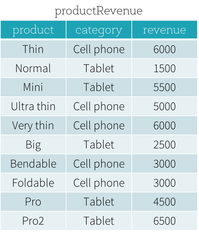
Suppose that we have a productRevenue table as shown below.

We want to answer two questions:

1. What are the best-selling and the second best-selling products in every category?
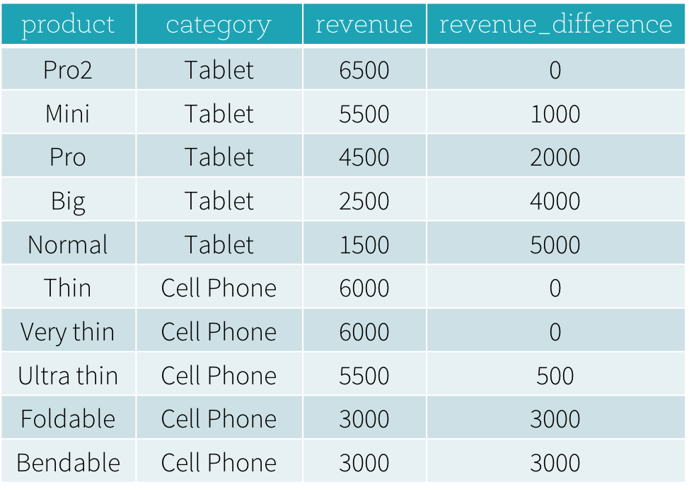
2. What is the difference between the revenue of each product and the revenue of the best-selling product in the same category of that product?

To answer the first question “What are the best-selling and the second best-selling products in every category?”, we need to rank products in a category based on their revenue, and to pick the best selling and the second best-selling products based the ranking. Below is the SQL query used to answer this question by using window function dense_rank (we will explain the syntax of using window functions in next section).

SELECT
  product,
  category,
  revenue
FROM (
  SELECT
    product,
    category,
    revenue,
    dense_rank() OVER (PARTITION BY category ORDER BY revenue DESC) as rank
  FROM productRevenue) tmp
WHERE
  rank 

The result of this query is shown below. Without using window functions, it is very hard to express the query in SQL, and even if a SQL query can be expressed, it is hard for the underlying engine to efficiently evaluate the query.

import sys from pyspark.sql.window import Window import pyspark.sql.functions as func windowSpec = \ Window .partitionBy(df['category']) \ .orderBy(df['revenue'].desc()) \ .rangeBetween(-sys.maxsize, sys.maxsize) dataFrame = sqlContext.table("productRevenue") revenue_difference = \ (func.max(dataFrame['revenue']).over(windowSpec) - dataFrame['revenue']) dataFrame.select( dataFrame['product'], dataFrame['category'], dataFrame['revenue'], revenue_difference.alias("revenue_difference")) 

The result of this program is shown below. Without using window functions, users have to find all highest revenue values of all categories and then join this derived data set with the original productRevenue table to calculate the revenue differences.

Using Window Functions

Spark SQL supports three kinds of window functions: ranking functions, analytic functions, and aggregate functions. The available ranking functions and analytic functions are summarized in the table below. For aggregate functions, users can use any existing aggregate function as a window function.

To use window functions, users need to mark that a function is used as a window function by either

• Adding an OVER clause after a supported function in SQL, e.g. avg(revenue) OVER (...); or
• Calling the over method on a supported function in the DataFrame API, e.g. rank().over(...).

Once a function is marked as a window function, the next key step is to define the Window Specification associated with this function. A window specification defines which rows are included in the frame associated with a given input row. A window specification includes three parts:

1. Partitioning Specification: controls which rows will be in the same partition with the given row. Also, the user might want to make sure all rows having the same value for  the category column are collected to the same machine before ordering and calculating the frame.  If no partitioning specification is given, then all data must be collected to a single machine.
2. Ordering Specification: controls the way that rows in a partition are ordered, determining the position of the given row in its partition.
3. Frame Specification: states which rows will be included in the frame for the current input row, based on their relative position to the current row.  For example, "the three rows preceding the current row to the current row" describes a frame including the current input row and three rows appearing before the current row.

In SQL, the PARTITION BY and ORDER BY keywords are used to specify partitioning expressions for the partitioning specification, and ordering expressions for the ordering specification, respectively. The SQL syntax is shown below.

OVER (PARTITION BY ... ORDER BY ...)

In the DataFrame API, we provide utility functions to define a window specification. Taking Python as an example, users can specify partitioning expressions and ordering expressions as follows.

from pyspark.sql.window import Window
windowSpec = \
  Window \
    .partitionBy(...) \
    .orderBy(...)

In addition to the ordering and partitioning, users need to define the start boundary of the frame, the end boundary of the frame, and the type of the frame, which are three components of a frame specification.

There are five types of boundaries, which are UNBOUNDED PRECEDING, UNBOUNDED FOLLOWING, CURRENT ROW, PRECEDING, and FOLLOWING. UNBOUNDED PRECEDING and UNBOUNDED FOLLOWING represent the first row of the partition and the last row of the partition, respectively. For the other three types of boundaries, they specify the offset from the position of the current input row and their specific meanings are defined based on the type of the frame. There are two types of frames, ROW frame and RANGE frame.

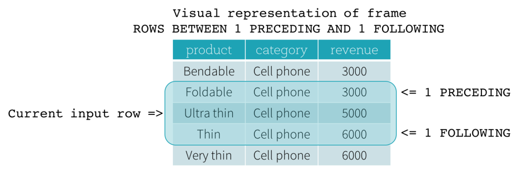
ROW frame

ROW frames are based on physical offsets from the position of the current input row, which means that CURRENT ROW, PRECEDING, or FOLLOWING specifies a physical offset. If CURRENT ROW is used as a boundary, it represents the current input row. PRECEDING and FOLLOWING describes the number of rows appear before and after the current input row, respectively. The following figure illustrates a ROW frame with a 1 PRECEDING as the start boundary and 1 FOLLOWING as the end boundary (ROWS BETWEEN 1 PRECEDING AND 1 FOLLOWING in the SQL syntax).

RANGE frame

RANGE frames are based on logical offsets from the position of the current input row, and have similar syntax to the ROW frame. A logical offset is the difference between the value of the ordering expression of the current input row and the value of that same expression of the boundary row of the frame. Because of this definition, when a RANGE frame is used, only a single ordering expression is allowed. Also, for a RANGE frame, all rows having the same value of the ordering expression with the current input row are considered as same row as far as the boundary calculation is concerned.

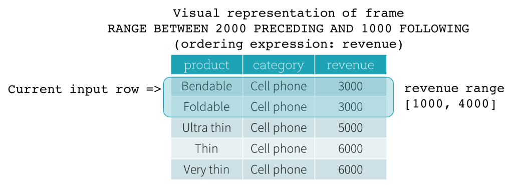
Now, let’s take a look at an example. In this example, the ordering expressions is revenue; the start boundary is 2000 PRECEDING; and the end boundary is 1000 FOLLOWING (this frame is defined as RANGE BETWEEN 2000 PRECEDING AND 1000 FOLLOWING in the SQL syntax). The following five figures illustrate how the frame is updated with the update of the current input row. Basically, for every current input row, based on the value of revenue, we calculate the revenue range [current revenue value - 2000, current revenue value + 1000]. All rows whose revenue values fall in this range are in the frame of the current input row.

In summary, to define a window specification, users can use the following syntax in SQL.

OVER (PARTITION BY ... ORDER BY ... frame_type BETWEEN start AND end)

Here, frame_type can be either ROWS (for ROW frame) or RANGE (for RANGE frame); start can be any of UNBOUNDED PRECEDING, CURRENT ROW, PRECEDING, and FOLLOWING; and end can be any of UNBOUNDED FOLLOWING, CURRENT ROW, PRECEDING, and FOLLOWING.

In the Python DataFrame API, users can define a window specification as follows.

from pyspark.sql.window import Window
# Defines partitioning specification and ordering specification.
windowSpec = \
  Window \
    .partitionBy(...) \
    .orderBy(...)
# Defines a Window Specification with a ROW frame.
windowSpec.rowsBetween(start, end)
# Defines a Window Specification with a RANGE frame.
windowSpec.rangeBetween(start, end)

What’s next?

Since the release of Spark 1.4, we have been actively working with community members on optimizations that improve the performance and reduce the memory consumption of the operator evaluating window functions. Some of these will be added in Spark 1.5, and others will be added in our future releases. Besides performance improvement work, there are two features that we will add in the near future to make window function support in Spark SQL even more powerful. First, we have been working on adding Interval data type support for Date and Timestamp data types (SPARK-8943). With the Interval data type, users can use intervals as values specified in PRECEDING and FOLLOWING for RANGE frame, which makes it much easier to do various time series analysis with window functions. Second, we have been working on adding the support for user-defined aggregate functions in Spark SQL (SPARK-3947). With our window function support, users can immediately use their user-defined aggregate functions as window functions to conduct various advanced data analysis tasks.

To try out these Spark features, get a free trial of Databricks or use the Community Edition.

Acknowledgements

The development of the window function support in Spark 1.4 is is a joint work by many members of the Spark community. In particular, we would like to thank Wei Guo for contributing the initial patch.