Amplify Insights into Your Industry With Geospatial Analytics

Data science is becoming commonplace and most companies are leveraging analytics and business intelligence to help make data-driven business decisions. But are you supercharging your analytics and decision-making with geospatial data? Location intelligence, and specifically geospatial analytics, can help uncover important regional trends and behavior that impact your business. This goes beyond looking at location data aggregated by zip codes, which interestingly in the US and in other parts of the world is not a good representation of a geographic boundary.

Are you a retailer who’s trying to figure out where to set up your next store or understand foot traffic that your competitors are getting in the same neighborhood? Or are you looking at real estate trends in the region to guide your next best investment? Do you deal with logistics and supply chain data and have to determine where the warehouses and fuel stops are located? Or do you need to identify network or service hot spots so you can adjust supply to meet demand? These use cases all have one point in common -- you can run a point-in-polygon operation to associate these latitude and longitude coordinates to their respective geographic geometries.

Technical implementation

The usual way of implementing a point-in-polygon operation would be to use a SQL function like st_intersects or st_contains from PostGIS, the open-source geographic information system(GIS) project. You could also use a few Apache Spark™  packages like Apache Sedona (previously known as Geospark) or Geomesa that offer similar functionality executed in a distributed manner, but these functions typically involve an expensive geospatial join that will take a while to run. In this blog post, we will take a look at how H3 can be used with Spark to help accelerate a large point-in-polygon problem, which is arguably one of the most common geospatial workloads that many will benefit from.

We introduced Uber’s H3 library in a past blog post. As a recap, H3 is a geospatial grid system that approximates geo features such as polygons or points with a fixed set of identifiable hexagonal cells. This can help scale large or computationally expensive big data workloads.

In our example, the WKT dataset that we are using contains MultiPolygons that may not work well with H3’s polyfill implementation. To ensure that our pipeline returns accurate results, we will need to split the MultiPolygons into individual Polygons.

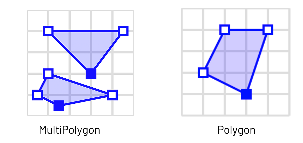
"SFA MultiPolygon" by  Mwtoews is licensed under CC BY-SA 3.0

%scala
import org.locationtech.jts.geom.GeometryFactory
import scala.collection.mutable.ArrayBuffer

def getPolygon = udf((geometry: Geometry)=>{
    var numGeometries = geometry.getNumGeometries()
    var polygonArrayBuffer = ArrayBuffer[Geometry]()
    for( geomIter 

After splitting the polygons, the next step is to create functions that define an H3 index for both your points and polygons. To scale this with Spark, you need to wrap your Python or Scala functions into Spark UDFs.

%scala
val res = 7 //the resolution of the H3 index, 1.2km
val points = df
    .withColumn("h3index", hex(geoToH3(col("pickup_latitude"), col("pickup_longitude"), lit(res))))

points.createOrReplaceTempView("points")

val polygons = wktDF
    .withColumn("h3index", multiPolygonToH3(col("the_geom"), lit(res)))
    .withColumn("h3", explode($"h3index"))
    .withColumn("h3", hex($"h3"))

polygons.createOrReplaceTempView("polygons")

H3 supports resolutions 0 to 15, with 0 being a hexagon with a length of about 1,107 km and 15 being a fine-grained hexagon with a length of about 50 cm. You should pick a resolution that is ideally a multiple of the number of unique Polygons in your dataset. In this example, we go with resolution 7.

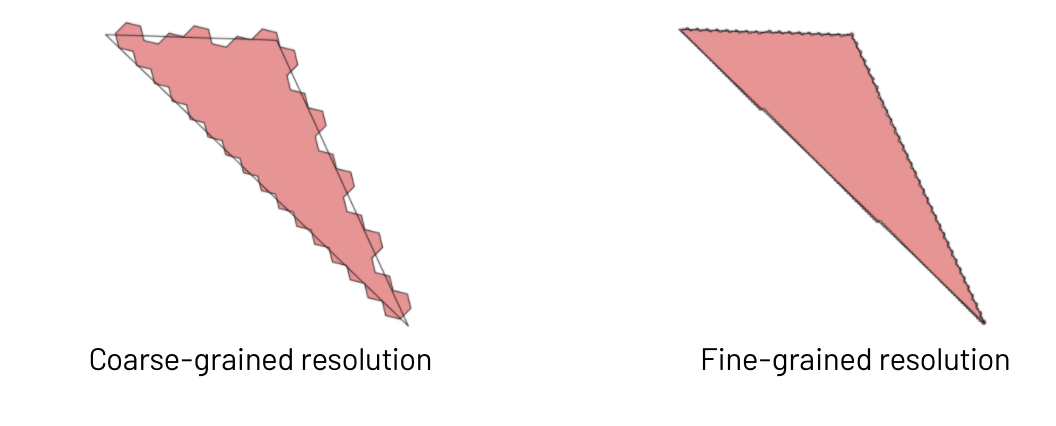
One thing to note here is that using H3 for a point-in-polygon operation will give you approximated results and we are essentially trading off accuracy for speed. Choosing a coarse-grained resolution may mean that you lose some accuracy at the polygon boundary, but your query will run really quickly. Picking a fine-grained resolution will give you better accuracy but will also increase the computational cost of the upcoming join query since you will have many more unique hexagons to join on. Picking the right resolution is a bit of an art, and you should consider how exact you need your results to be. Considering that your GPS points may not be that precise, perhaps forgoing some accuracy for speed is acceptable.

With the points and polygons indexed with H3, it’s time to run the join query. Instead of running a spatial command like st_intersects or st_contains here, which would trigger an expensive spatial join, you can now run a simple Spark inner join on the H3 index column. Your point-in-polygon query can now run in the order of minutes on billions of points and thousands or millions of polygons.

%sql
SELECT *
FROM
    Points p
    INNER JOIN
    Polygons s
    ON p.h3 = s.h3

If you require more accuracy, another possible approach here is to leverage the H3 index to reduce the number of rows passed into the geospatial join. Your query would look something like this, where your st_intersects() or st_contains() command would come from 3rd party packages like Geospark or Geomesa:

%sql
SELECT * 
FROM 
    points p 
    INNER JOIN
    shape s 
    ON p.h3 = s.h3
WHERE st_intersects(st_makePoint(p.pickup_longitude, p.pickup_latitude), s.the_geom);    

Potential optimizations

It’s common to run into data skews with geospatial data. For example, you might receive more cell phone GPS data points from urban areas compared to sparsely populated areas. This means that there may be certain H3 indices that have way more data than others, and this introduces skew in our Spark SQL join. This is true as well for the dataset in our notebook example where we see a huge number of taxi pickup points in Manhattan compared to other parts of New York. We can leverage skew hints here to help with the join performance.

First, determine what your top H3 indices are.

display(points.groupBy("h3").count().orderBy($"count".desc))

Then, re-run the join query with a skew hint defined for your top index or indices. You could also try broadcasting the polygon table if it’s small enough to fit in the memory of your worker node.

SELECT /*+ SKEW('points_with_id_h3', 'h3', ('892A100C68FFFFF')), BROADCAST(polygons) */ 
*
FROM
    points p
    INNER JOIN
    Polygons s
    ON p.h3 = s.h3

Also, don’t forget to have the table with more rows on the left side of the join. This reduces shuffle during the join and can greatly improve performance.

Do note that with Spark 3.0’s new Adaptive Query Execution (AQE), the need to manually broadcast or optimize for skew would likely go away. If your favorite geospatial package supports Spark 3.0 today, do check out how you could leverage AQE to accelerate your workloads!

Data visualization

A good way to visualize H3 hexagons would be to use Kepler.gl, which was also developed by Uber. There’s a PyPi library for Kepler.gl that you could leverage within your Databricks notebook. Do refer to this notebook example if you’re interested in giving it a try.

The Kepler.gl library runs on a single machine. This means that you will need to sample down large datasets before visualizing. You can create a random sample of the results of your point-in-polygon join and convert it into a Pandas dataframe and pass that into Kepler.gl.

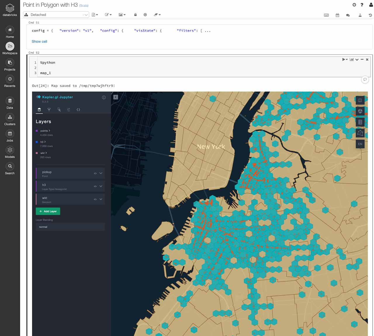
Now you can explore your points, polygons, and hexagon grids on a map within a Databricks notebook. This is a great way to verify the results of your point-in-polygon mapping as well!

Try the notebook

Please Note: The notebook may not display correctly when viewed in the browser. For best results, please download and run it in your Databricks Workspace.