Design Patterns for Batch Processing in Financial Services

Introduction

Financial services institutions (FSIs) around the world are facing unprecedented challenges ranging from market volatility and political uncertainty to changing legislation and regulations. Businesses are forced to accelerate digital transformation programs; automating critical processes to reduce operating costs and improve response times. However, with data typically scattered across multiple systems, accessing the information required to execute on these initiatives tends to be easier said than done.

Architecting an ecosystem of services able to support the plethora of data-driven use cases in this digitally transformed business can, however, seem to be an impossible task. This blog will focus on one crucial aspect of the modern data stack: batch processing. A seemingly outdated paradigm, we'll see why batch processing remains a vital and highly viable component of the data architecture. And we'll see how Databricks can help FSIs navigate some of the crucial challenges faced when building infrastructure to support these scheduled or periodic workflows.

Why batch ingestion matters

Over the last two decades, the global shift towards an instant society has forced organizations to rethink the operating and engagement model. A digital-first strategy is no longer optional but vital for survival. Customer needs and demands are changing and evolving faster than ever. This desire for instant gratification is driving an increased focus on building capabilities that support real-time processing and decisioning. One might ask whether batch processing is still relevant in this new dynamic world.

While real-time systems and streaming services can help FSIs remain agile in addressing the volatile market conditions at the edge, they do not typically meet the requirements of back-office functions. Most business decisions are not reactive but rather, require considered, strategic reasoning. By definition, this approach requires a systematic review of aggregate data collected over a period of time. Batch processing in this context still provides the most efficient and cost-effective method for processing large, aggregate volumes of data. Additionally, batch processing can be done offline, reducing operating costs and providing greater control over the end-to-end process.

The world of finance is changing, but across the board incumbents and startups continue to rely heavily on batch processing to power core business functions. Whether for reporting and risk management or anomaly detection and surveillance, FSIs require batch processing to reduce human error, increase the speed of delivery, and reduce operating costs.

Getting started

Starting with a 30,000-ft view, most FSIs will have a multitude of data sources scattered across on-premises systems, cloud-based services and even third-party applications. Building a batch ingestion framework that caters for all these connections require complex engineering and can quickly become a burden on maintenance teams. And that's even before considering things like change data capture (CDC), scheduling, and schema evolution. In this section, we will demonstrate how the Databricks Lakehouse for Financial Services (LFS) and its ecosystem of partners can be leveraged to address these key challenges and greatly simplify the overall architecture.

The Databricks Lakehouse was designed to provide a unified platform that supports all analytical and scientific data workloads. Figure 1 shows the reference architecture for a decoupled design that allows easy integration with other platforms that support the modern data ecosystem. The lakehouse makes it easy to construct ingestion and serving layers that operate irrespective of the data's source, volume, velocity, and destination.

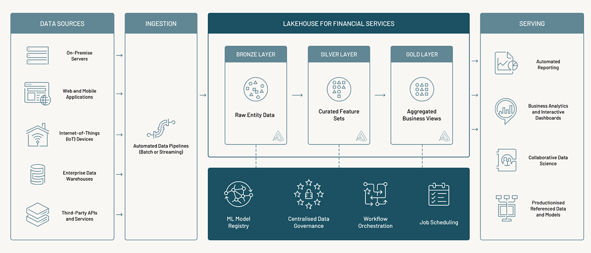
To demonstrate the power and efficiency of the LFS, we turn to the world of insurance. We consider the basic reporting requirements for a typical claims workflow. In this scenario, the organization might be interested in the key metrics driven by claims processes. For example:

• Number of active policies
• Number of claims
• Value of claims
• Total exposure
• Loss ratio

Additionally, the business might want a view of potentially suspicious claims and a breakdown by incident type and severity. All these metrics are easily calculable from two key sources of data: 1) the book of policies and 2) claims filed by customers. The policy and claims records are typically stored in a combination of enterprise data warehouses (EDWs) and operational databases. The main challenge becomes connecting to these sources and ingesting data into our lakehouse, where we can leverage the power of Databricks to calculate the desired outputs.

Luckily, the flexible design of the LFS makes it easy to leverage best-in-class products from a range of SaaS technologies and tools to handle specific tasks. One possible solution for our claims analytics use case would be to use Fivetran for the batch ingestion plane. Fivetran provides a simple and secure platform for connecting to numerous data sources and delivering data directly to the Databricks Lakehouse. Additionally, it offers native support for CDC, schema evolution and workload scheduling. In Figure 2, we show the technical architecture of a practical solution for this use case.

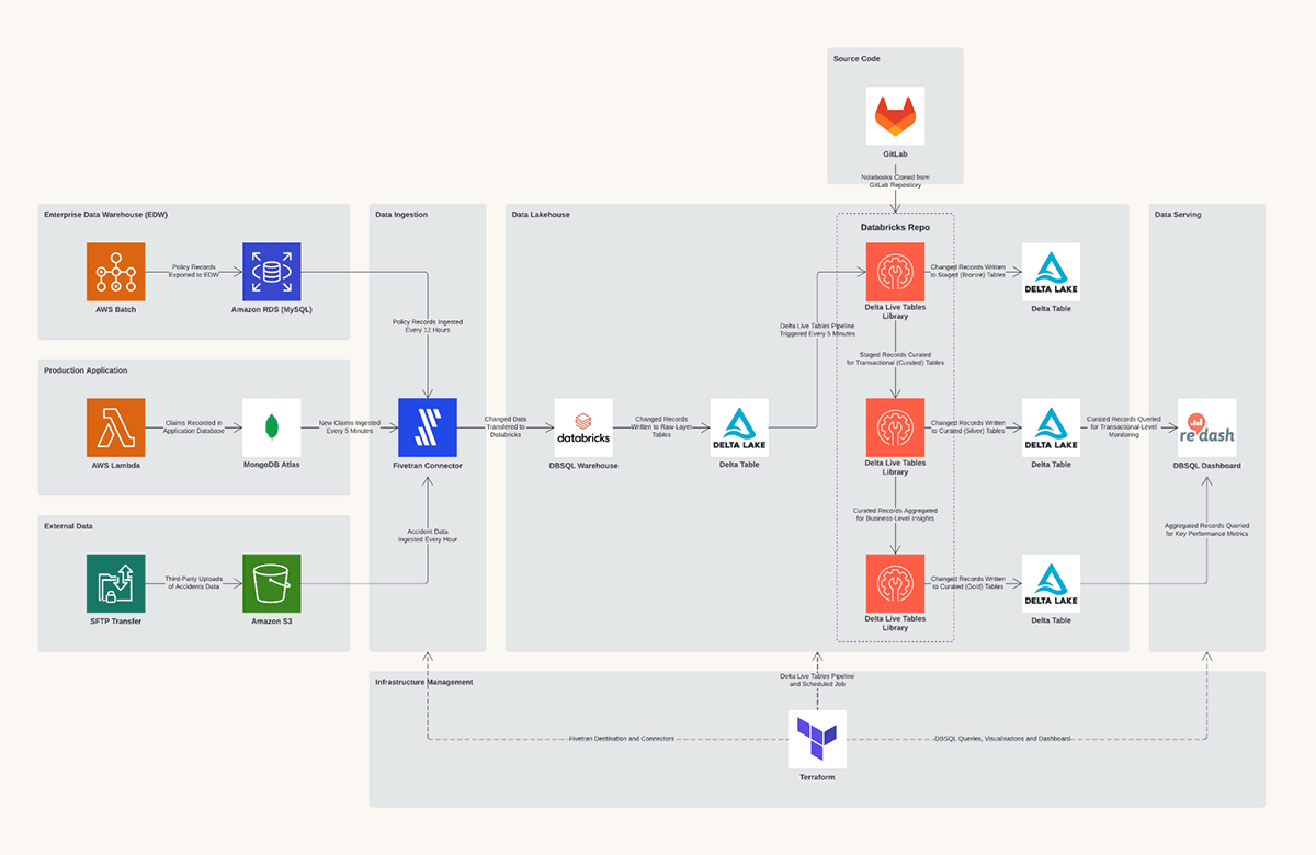
Once the data is ingested and delivered to the LFS, we can use Delta Live Tables (DLT) for the entire engineering workflow. DLT provides a simple, scalable declarative framework for automating complex workflows and enforcing data quality controls. The outputs from our DLT workflow, our curated and aggregated assets, can be interrogated using Databricks SQL (DB SQL). DB SQL brings data warehousing to the LFS to power business-critical analytical workloads. Results from DB SQL queries can be packaged in easy-to-consume dashboards and served to business users.

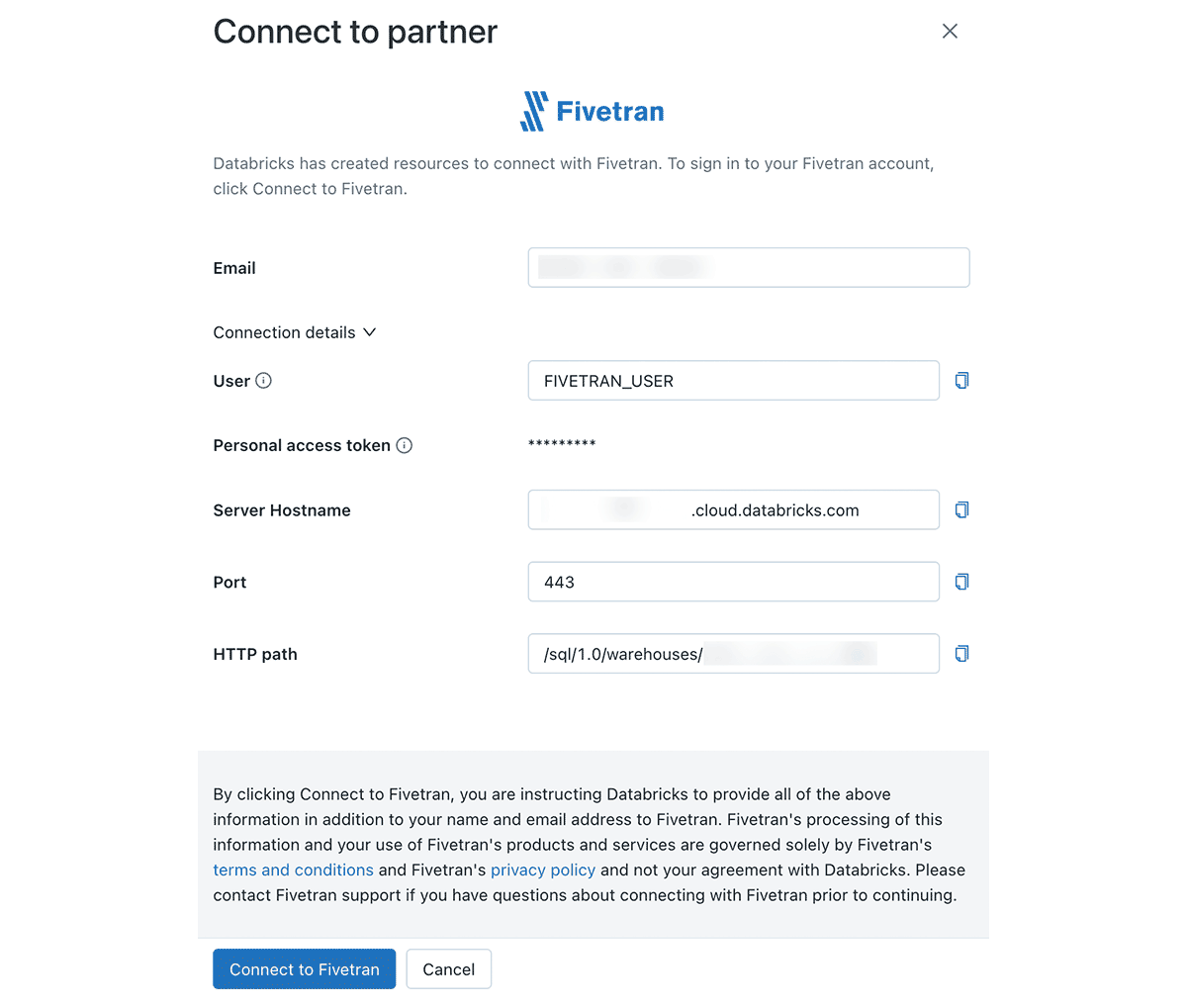
Step 1: Creating the ingestion layer

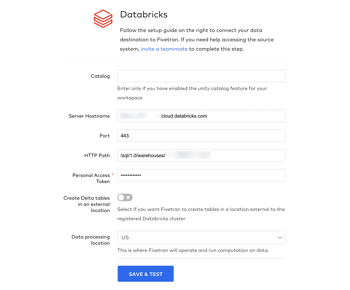
Setting up an ingestion layer with Fivetran requires a two-step process. First, configuring a so-called destination where data will be delivered, and second, establishing one or more connections with the source systems. The Partner Connect interface takes care of the first step with a simple, guided interface to connect Fivetran with a Databricks Warehouse. Fivetran will use the warehouse to convert raw source data to Delta Tables and store the results in the Databricks Lakehouse. Figures 3 and 4 show steps from the Partner Connect and Fivetran interfaces to configure a new destination.

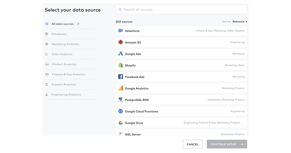
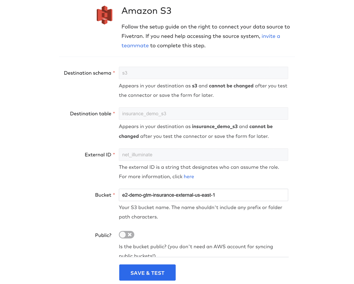
For the next step, we move to the Fivetran interface. From here, we can easily create and configure connections to several different source systems (please refer to the official documentation for a complete list of all supported connections). In our example, we consider three sources of data: 1) policy records stored in an Operational Data Store (ODS) or Enterprise Data Warehosue (EDW), 2) claims records stored in an operational database, and 3) external data delivered to blob storage. As such, we require three different connections to be configured in Fivetran. For each of these, we can follow Fivetran's simple guided process to set up a connection with the source system. Figures 5 and 6 show how to configure new connections to data sources.

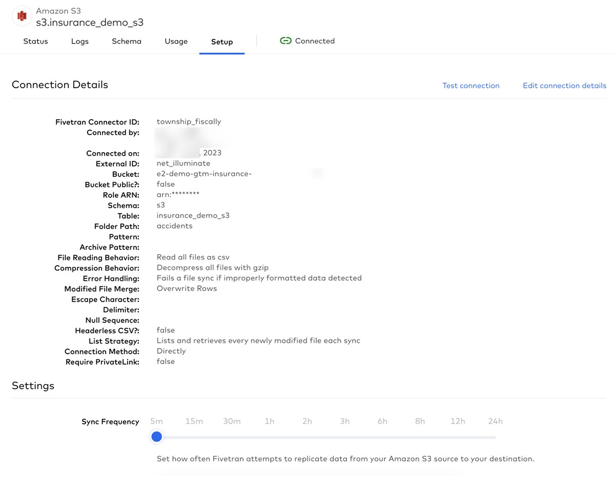
Connections can further be configured once they have been validated. One important option to set is the frequency with which Fivetran will interrogate the source system for new data. In Figure 7, we can see how easy Fivetran has made it to set the sync frequency with intervals ranging from 5 minutes to 24 hours.

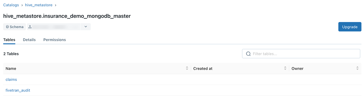
Fivetran will immediately interrogate and ingest data from source systems once a connection is validated. Data is stored as Delta tables and can be viewed from within Databricks through the DB SQL Data Explorer. By default, Fivetran will store all data under the Hive metastore. A new schema is created for each new connection, and each schema will contain at least two tables: one containing the data and another with logs from each attempted ingestion cycle (see Figure 8).

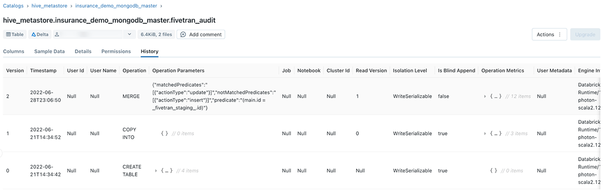
Having the data stored in Delta tables is a significant advantage. Delta Lake natively supports granular data versioning, meaning we can time travel through each ingestion cycle (see Figure 9). We can use DB SQL to interrogate specific versions of the data to analyze how the source records evolved.

It is important to note that if the source data contains semi-structured or unstructured values, those attributes will be flattened during the conversion process. This means that the results will be stored in grouped text-type columns, and these entities will have to be dissected and unpacked with DLT in the curation process to create separate attributes.

Step 2: Automating the workflow

With the data in the Databricks Lakehouse, we can use Delta Live Tables (DLT) to build a simple, automated data engineering workflow. DLT provides a declarative framework for specifying detailed feature engineering steps. Currently, DLT supports APIs for both Python and SQL. In this example, we will use Python APIs to build our workflow.

The most fundamental construct in DLT is the definition of a table. DLT interrogates all table definitions to create a comprehensive workflow for how data should be processed. For instance, in Python, tables are created using function definitions and the `dlt.table` decorator (see example of Python code below). The decorator is used to specify the name of the resulting table, a descriptive comment explaining the purpose of the table, and a collection of table properties.

@dlt.table(
   name             = "curated_claims",
   comment          = "Curated claim records",
   table_properties = {
       "layer": "silver",
       "pipelines.autoOptimize.managed": "true",
       "delta.autoOptimize.optimizeWrite": "true",
       "delta.autoOptimize.autoCompact": "true"
   }
)
def curate_claims():
   # Read the staged claim records into memory
   staged_claims = dlt.read("staged_claims")
   # Unpack all nested attributes to create a flattened table structure
   curated_claims = unpack_nested(df = staged_claims, schema = schema_claims)

   ...

Instructions for feature engineering are defined inside the function body using standard PySpark APIs and native Python commands. The following example shows how PySpark joins claims records with data from the policies table to create a single, curated view of claims.

   ...   

   # Read the staged claim records into memory
   curated_policies = dlt.read("curated_policies")
   # Evaluate the validity of the claim
   curated_claims = curated_claims \
       .alias("a") \
       .join(
           curated_policies.alias("b"),
           on  = F.col("a.policy_number") == F.col("b.policy_number"),
           how = "left"
       ) \
       .select([F.col(f"a.{c}") for c in curated_claims.columns] + [F.col(f"b.{c}").alias(f"policy_{c}")  for c in ("effective_date", "expiry_date")]) \
       .withColumn(
           # Calculate the number of months between coverage starting and the claim being filed
           "months_since_covered", F.round(F.months_between(F.col("claim_date"), F.col("policy_effective_date")))
       ) \
       .withColumn(
           # Check if the claim was filed before the policy came into effect
           "claim_before_covered", F.when(F.col("claim_date") < F.col("policy_effective_date"), F.lit(1)).otherwise(F.lit(0))
       ) \
       .withColumn(
           # Calculate the number of days between the incident occurring and the claim being filed
           "days_between_incident_and_claim", F.datediff(F.col("claim_date"), F.col("incident_date"))
       )
  
   # Return the curated dataset
   return curated_claims

One significant advantage of DLT is the ability to specify and enforce data quality standards. We can set expectations for each DLT table with detailed data quality constraints that should be applied to the contents of the table. Currently, DLT supports expectations for three different scenarios:

Expectations can be defined with one or more data quality constraints. Each constraint requires a description and a Python or SQL expression to evaluate. Multiple constraints can be defined using the expect_all, expect_all_or_drop, and expect_all_or_fail decorators. Each decorator expects a Python dictionary where the keys are the constraint descriptions, and the values are the respective expressions. The example below shows multiple data quality constraints for the retain and drop scenarios described above.

@dlt.expect_all({
   "valid_driver_license": "driver_license_issue_date > (current_date() - cast(cast(driver_age AS INT) AS INTERVAL YEAR))",
   "valid_claim_amount": "total_claim_amount > 0",
   "valid_coverage": "months_since_covered > 0",
   "valid_incident_before_claim": "days_between_incident_and_claim > 0"
})
@dlt.expect_all_or_drop({
   "valid_claim_number": "claim_number IS NOT NULL",
   "valid_policy_number": "policy_number IS NOT NULL",
   "valid_claim_date": "claim_date < current_date()",
   "valid_incident_date": "incident_date < current_date()",
   "valid_incident_hour": "incident_hour between 0 and 24",
   "valid_driver_age": "driver_age > 16",
   "valid_effective_date": "policy_effective_date < current_date()",
   "valid_expiry_date": "policy_expiry_date <= current_date()"
})
def curate_claims():
    ...

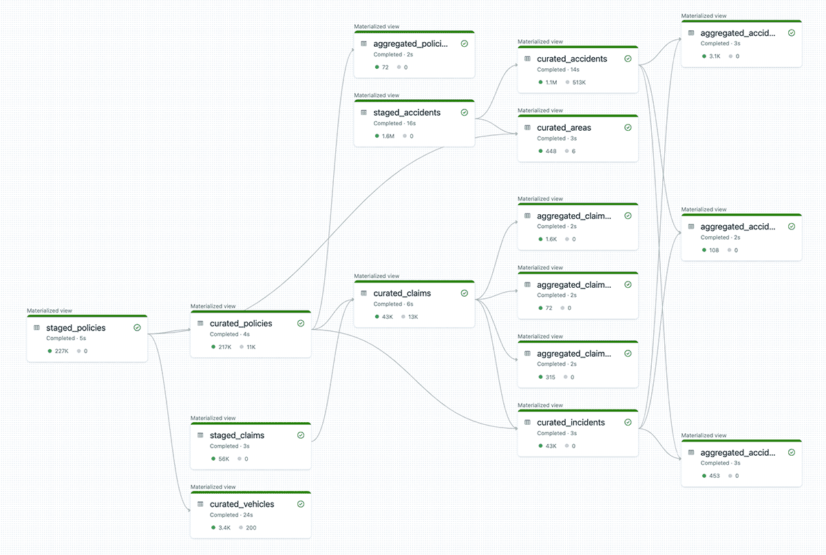
We can use more than one Databricks Notebook to declare our DLT tables. Assuming we follow the medallion architecture, we can, for example, use different notebooks to define tables comprising the bronze, silver, and gold layers. The DLT framework can digest instructions defined across multiple notebooks to create a single workflow; all inter-table dependencies and relationships are processed and considered automatically. Figure 10 shows the complete workflow for our claims example. Starting with three source tables, DLT builds a comprehensive pipeline that delivers thirteen tables for business consumption.

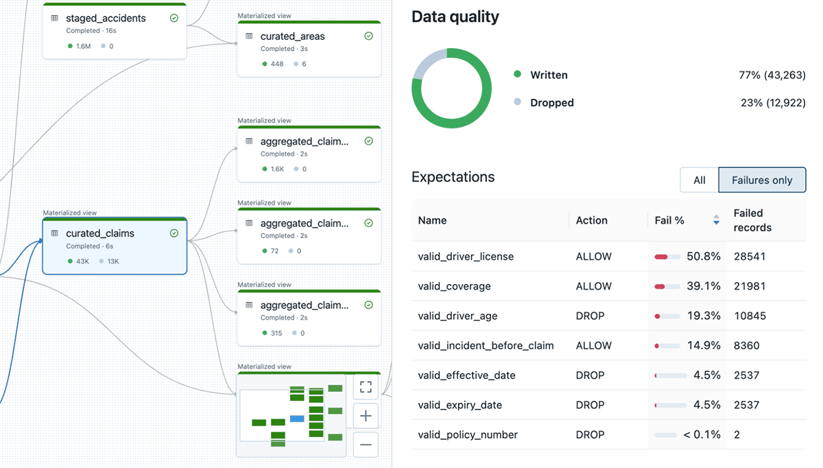
Results for each table can be inspected by selecting the desired entity. Figure 11 provides an example of the results of the curated claims table. DLT provides a high-level overview of the results from the data quality controls:

Results from the data quality expectations can be analyzed further by querying the event log. The event log contains detailed metrics about all expectations defined for the workflow pipeline. The query below provides an example for viewing key metrics from the last pipeline update, including the number of records that passed or failed expectations:

SELECT
  row_expectations.dataset AS dataset,
  row_expectations.name AS expectation,
  SUM(row_expectations.passed_records) AS passing_records,
  SUM(row_expectations.failed_records) AS failing_records
FROM
  (
    SELECT
      explode(
        from_json(
          details :flow_progress :data_quality :expectations,
          "array<struct<name: string, dataset: string, passed_records: int, failed_records: int>>"
        )
      ) row_expectations
    FROM
      event_log_raw
    WHERE
      event_type = 'flow_progress'
      AND origin.update_id = '${latest_update.id}'
  )
GROUP BY
  row_expectations.dataset,
  row_expectations.name;

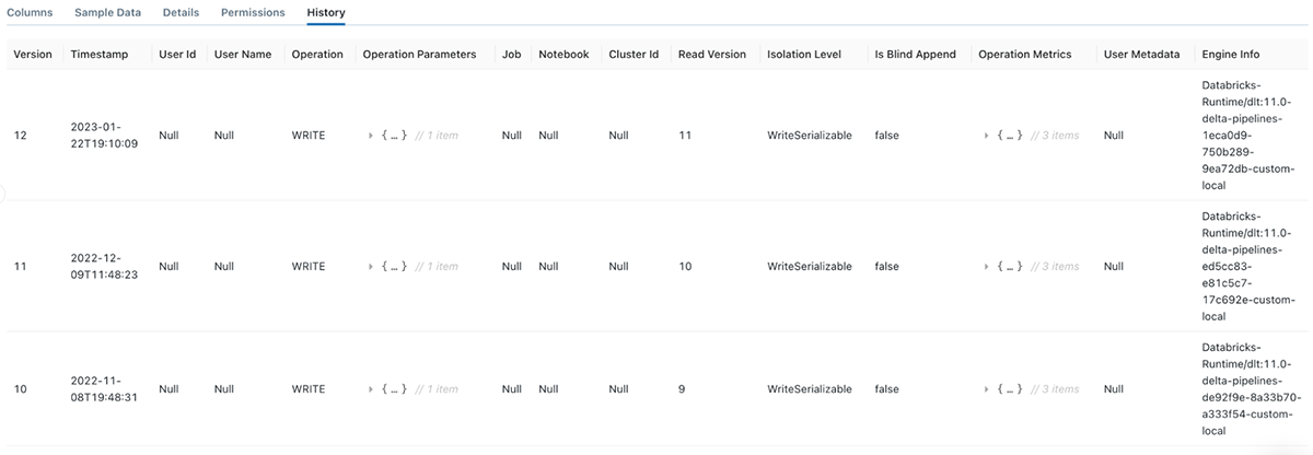
Again, we can view the complete history of changes made to each DLT table by looking at the Delta history logs (see Figure 12). It allows us to understand how tables evolve over time and investigate complete threads of updates if a pipeline fails.

We can further use change data capture (CDC) to update tables based on changes in the source datasets. DLT CDC supports updating tables with slow-changing dimensions (SCD) types 1 and 2.

We have one of two options for our batch process to trigger the DLT pipeline. We can use the Databricks Auto Loader to incrementally process new data as it arrives in the source tables or create scheduled jobs that trigger at set times or intervals. In this example, we opted for the latter with a scheduled job that executes the DLT pipeline every five minutes.

Operationalizing the outputs

The ability to incrementally process data efficiently is only half of the equation. Results from the DLT workflow must be operationalized and delivered to business users. In our example, we can consume outputs from the DLT pipeline through ad hoc analytics or prepacked insights made available through an interactive dashboard.

Ad hoc analytics

Databricks SQL (or DB SQL) provides an efficient, cost-effective data warehouse on top of the Databricks Lakehouse platform. It allows us to run our SQL workloads directly against the source data with up to 12x better price/performance than its alternatives.

We can leverage DB SQL to perform specific ad hoc queries against our curated and aggregated tables. We might, for example, run a query against the curated policies table that calculates the total exposure. The DB SQL query editor provides a simple, easy-to-use interface to build and execute such queries (see example below).

SELECT
  round(curr.total_exposure, 0) AS total_exposure,
  round(prev.total_exposure, 0) AS previous_exposure
FROM
  (
    SELECT
      sum(sum_insured) AS total_exposure
    FROM
      insurance_demo_lakehouse.curated_policies
    WHERE
      expiry_date > '{{ date.end }}'
      AND (effective_date <= '{{ date.start }}'
        OR (effective_date BETWEEN '{{ date.start }}' AND '{{ date.end }}'))
  ) curr
  JOIN
  (
    SELECT
      ...

We can also use the DB SQL query editor to run queries against different versions of our Delta tables. For example, we can query a view of the aggregated claims records for a specific date and time (see example below). We can further use DB SQL to compare results from different versions to analyze only the changed records between those states.

SELECT
  *
FROM
  insurance_demo_lakehouse.aggregated_claims_weekly TIMESTAMP AS OF '2022-06-05T17:00:00';

DB SQL offers the option to use a serverless compute engine, eliminating the need to configure, manage or scale cloud infrastructure while maintaining the lowest possible cost. It also integrates with alternative SQL workbenches (e.g., DataGrip), allowing analysts to use their favorite tools to explore the data and generate insights.

Business insights

Finally, we can use DB SQL queries to create rich visualizations on top of our query results. These visualizations can then be packaged and served to end users through interactive dashboards (see Figure 13).

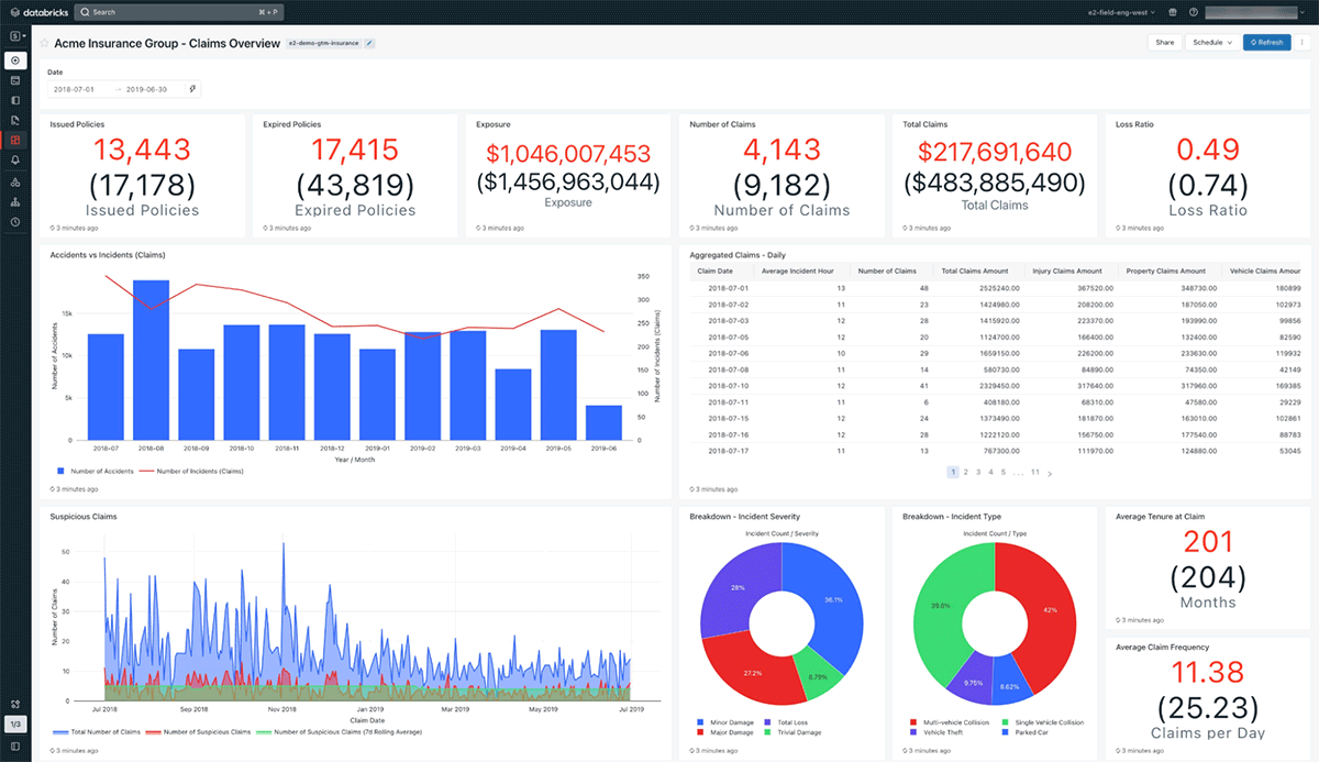
For our use case, we created a dashboard with a collection of key metrics, rolling calculations, high-level breakdowns, and aggregate views. The dashboard provides a complete summary of our claims process at a glance. We also added the option to specify specific date ranges. DB SQL supports a range of query parameters that can substitute values into a query at runtime. These query parameters can be defined at the dashboard level to ensure all related queries are updated accordingly.

DB SQL integrates with numerous third-party analytical and BI tools like Power BI, Tableau and Looker. Like we did for Fivetran, we can use Partner Connect to link our external platform with DB SQL. This allows analysts to build and serve dashboards in the platforms that the business prefers without sacrificing the performance of DB SQL and the Databricks Lakehouse.

Conclusion

As we move into this fast-paced, volatile modern world of finance, batch processing remains a vital part of the modern data stack, able to hold its own against the features and benefits of streaming and real-time services. We've seen how we can use the Databricks Lakehouse for Financial Services and its ecosystem of partners to architect a simple, scalable, and extensible framework that supports complex batch-processing workloads with a practical example in insurance claims processing. With Delta Live Tables (DLT) and Databricks SQL (DB SQL), we can build a data platform with an architecture that scales infinitely, is easy to extend to address changing requirements, and will withstand the test of time.

To learn more about the sample pipeline described, including the infrastructure setup and configuration used, please refer to this GitHub repository or watch this demo video..