Fine Grained Forecasting With R
by Divya Saini and Bryan Smith
Demand forecasting is foundational to most organizations' planning functions. By anticipating consumer demand for goods and services, activities across marketing and up and down the supply chain can be aligned to ensure the right resources are in the right place at the right time and price, maximizing revenue and minimizing cost.
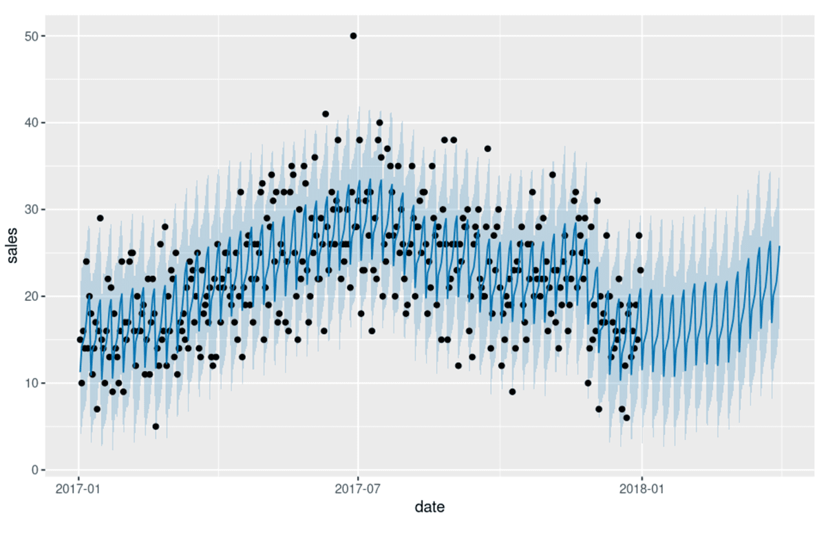
While the progression from forecast to plan and ultimately to execution is often far less orderly than the previous statement would imply, the process begins with the adoption of an accurate forecast. The expectation is never that the forecast will perfectly predict future demand but instead will provide a manageable range of likely outcomes around which the organization can plan its activities (Figure 1).
That said, many organizations struggle to produce forecasts sufficiently reliable for this purpose. One survey revealed inaccuracies of 20 to 40% across a range of industries. Other surveys report similar results with the consequence being an erosion of organizational trust and the continuation of planning activities based on expert opinion and gut feel.
The reasons behind this high level of inaccuracy vary, but often they come down to a lack of access to more sophisticated forecasting technology or the computational resources needed to apply them at scale. For decades, organizations have found themselves bound to the limitations of pre-built software solutions and forced to produce aggregate-level forecasts in order to deliver timely results. The forecasts produced often do a good job of presenting the macro-level patterns of demand but unable to capture localized variations where that demand is met (Figure 2).
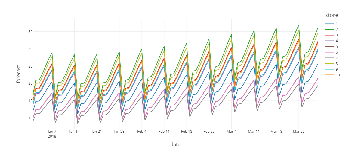
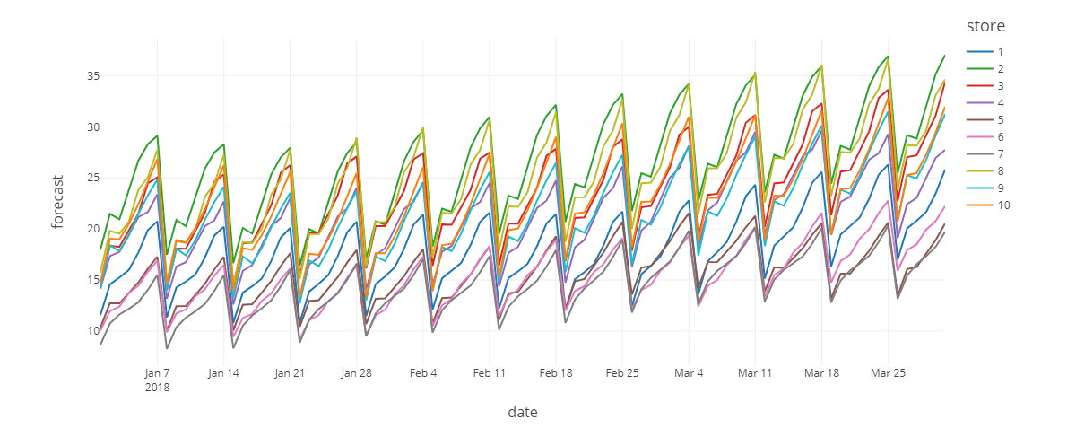
Figure 2. A comparison of an aggregated forecast allocated to the store-item level vs. a fine-grained forecast performed at the individual store-item level.
But with the emergence of data science as an enterprise capability, there is renewed interest across many organizations to revisit legacy forecasting practices. As noted in a far reaching examination of data and AI-driven innovation by McKinsey, "a 10 to 20% increase in forecasting accuracy translates into a potential 5% reduction of inventory costs and revenue increases of 2 to 3%." In an increasingly competitive economic climate, such benefits are providing ample incentive for organizations to explore new approaches.
The R language provides access to new forecasting techniques
Much of the interest in new and novel forecasting techniques is expressed through the community of R developers. Created in the mid-1990s as an open source language for statistical computing, R remains highly popular with statisticians and academics pushing the boundaries of a broad range of analytic techniques. With broad adoption across both graduate and undergraduate Data Science programs, many organizations are finding themselves flush with R development skills, making the language and the sophisticated packages it supports increasingly accessible.
The key to R's sustained success is its extensibility. While the core R language provides access to fundamental data management and analytic capabilities, most data scientists make heavy use of the broad portfolio of packages contributed by the practitioner community. The availability of forecasting-related packages in the R language is particularly notable, reflecting the widespread interest in innovation within this space.
The cloud provides access to the computational resources
But the availability of statistical software is just part of the challenge. To drive better forecasting outcomes, organizations need the ability to predict exactly how a product will behave in a given location, and this can often mean needing to produce multiple-millions of forecasts on a regular basis.
In prior periods, organizations struggled to provide the resources needed to turn around this volume of forecasts in a timely manner. To do so, organizations would need to secure large volumes of servers that would largely sit idle between forecasting cycles, and few could justify the expense.
However, with the emergence of the cloud, organizations now find themselves able to rent these resources for just those periods within which they are needed. Taking advantage of low cost storage options, forecast output can be persisted for consumption by analysts between forecasting cycles, making fine-grained forecasting at the store-item level suddenly viable for most organizations.
The challenge then is how best to acquire these resources when needed, distribute the work across them, persist the output and deprovision the computing resources in a timely manner. Past frameworks for such work were often complex and inflexible, but today we have Databricks.
Databricks brings together R functionality with cloud scalability
Databricks is a highly accessible platform for scalable data processing within the cloud. Through Databricks clusters, large volumes of virtual servers can be rapidly provisioned and deprovisioned to affect workloads big and small. Leveraging widely adopted languages such as Python, SQL and R, developers can work with data using simple constructs, allowing the underlying engine to abstract much of the complexity of the distributed work. That said, if we peer a bit behind the covers, we can find even greater opportunities to exploit Databricks, including ways that help us tackle the problem of producing very large volumes of forecasts leveraging R.
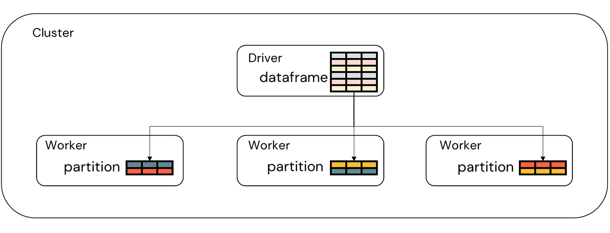
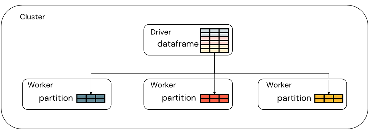
To get us started with this, consider that Databricks collects data within a Spark dataframe. To the developer, this dataframe appears as a singular object. However, the individual records accessible within the dataframe are in fact divided into smaller collections referred to as partitions. A given partition resides on a single worker node (server) within the Databricks cluster so while the dataframe is accessed as a singular object (on the primary/driver node), it is in fact a collection of non-overlapping partitions residing on the servers that make up the cluster (Figure 3).
Against the dataframe, a developer applies various data transformations. Under the covers, the Spark engine decides how these transformations are applied to the partitions. Some transformations such as the grouping of data ahead of an aggregation trigger the engine to rearrange the records in the dataframe into a new set of partitions within which all the records associated with a given key value reside. If you were, for example, to read historical sales data into a Spark dataframe and then group that data on a store and item key, then you would be left with one partition for each store-item combination within the dataset. And that's the key to tackling our fine-grained forecasting challenge (Figure 4).
By grouping all the records for a given store and item within a partition, we've isolated all the data we need to produce a store-item level forecast in one place. We can then write a function which treats the partition as an R dataframe, train a model against it and return predictions back as a new Spark dataframe object (Figure 5).
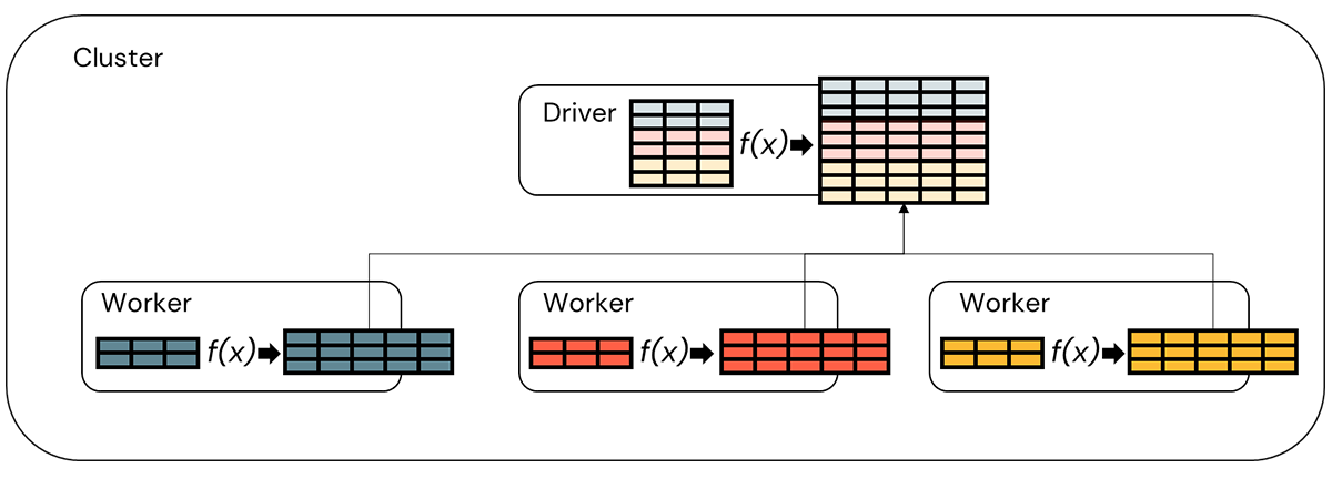
The R language provides us two options for doing this. Using the SparkR package, we can use the gapply function to group the data and apply a user-defined function to each partition. Using the SparklyR package, we can do the same thing using the spark_apply function. The choice of R packages, i.e. SparkR or SparklyR, to facilitate this work is really up to developer preference with SparkR providing more direct access to Spark functionality and SparklyR wrapping that functionality in an API more familiar to developers comfortable with the R dpylr package.
Want to see these two approaches in action? Then, please check out the Solution Accelerators.
Get the latest posts in your inbox
Subscribe to our blog and get the latest posts delivered to your inbox.