LLM Inference Performance Engineering: Best Practices
by Megha Agarwal, Asfandyar Qureshi, Nikhil Sardana, Linden Li, Julian Quevedo and Daya Khudia
In this blog post, the MosaicML engineering team shares best practices for how to capitalize on popular open source large language models (LLMs) for production usage. We also provide guidelines for deploying inference services built around these models to help users in their selection of models and deployment hardware. We have worked with multiple PyTorch-based backends in production; these guidelines are drawn from our experience with FasterTransformers, vLLM, NVIDIA's soon-to-be-released TensorRT-LLM, and others.
Understanding LLM Text Generation
Large Language Models (LLMs) generate text in a two-step process: "prefill", where the tokens in the input prompt are processed in parallel, and "decoding", where text is generated one 'token' at a time in an autoregressive manner. Each generated token is appended to the input and fed back into the model to generate the next token. Generation stops when the LLM outputs a special stop token or when a user-defined condition is met (e.g., some maximum number of tokens has been generated). If you'd like more background on how LLMs use decoder blocks, check out this blog post.
Tokens can be words or sub-words; the exact rules for splitting text into tokens vary from model to model. For instance, you can compare how Llama models tokenize text to how OpenAI models tokenize text. Although LLM inference providers often talk about performance in token-based metrics (e.g., tokens/second), these numbers are not always comparable across model types given these variations. For a concrete example, the team at Anyscale found that Llama 2 tokenization is 19% longer than ChatGPT tokenization (but still has a much lower overall cost). And researchers at HuggingFace also found that Llama 2 required ~20% more tokens to train over the same amount of text as GPT-4.
Important Metrics for LLM Serving
So, how exactly should we think about inference speed?
Our team uses four key metrics for LLM serving:
- Time To First Token (TTFT): How quickly users start seeing the model's output after entering their query. Low waiting times for a response are essential in real-time interactions, but less important in offline workloads. This metric is driven by the time required to process the prompt and then generate the first output token.
- Time Per Output Token (TPOT): Time to generate an output token for each user that is querying our system. This metric corresponds with how each user will perceive the "speed" of the model. For example, a TPOT of 100 milliseconds/tok would be 10 tokens per second per user, or ~450 words per minute, which is faster than a typical person can read.
- Latency: The overall time it takes for the model to generate the full response for a user. Overall response latency can be calculated using the previous two metrics: latency = (TTFT) + (TPOT) * (the number of tokens to be generated).
- Throughput: The number of output tokens per second an inference server can generate across all users and requests.
Our goal? The fastest time to first token, the highest throughput, and the quickest time per output token. In other words, we want our models to generate text as fast as possible for as many users as we can support.
Notably, there is a tradeoff between throughput and time per output token: if we process 16 user queries concurrently, we'll have higher throughput compared to running the queries sequentially, but we'll take longer to generate output tokens for each user.
If you have overall inference latency targets, here are some useful heuristics for evaluating models:
- Output length dominates overall response latency: For average latency, you can usually just take your expected/max output token length and multiply it by an overall average time per output token for the model.
- Input length is not significant for performance but important for hardware requirements: The addition of 512 input tokens increases latency less than the production of 8 additional output tokens in the MPT models. However, the need to support long inputs can make models harder to serve. For example, we recommend using the A100-80GB (or newer) to serve MPT-7B with its maximum context length of 2048 tokens.
- Overall latency scales sub-linearly with model size: On the same hardware, larger models are slower, but the speed ratio won't necessarily match the parameter count ratio. MPT-30B latency is ~2.5x that of MPT-7B latency. Llama2-70B latency is ~2x that of Llama2-13B latency.
We are often asked by prospective customers to provide an average inference latency. We recommend that before you anchor yourself to specific latency targets ("we need less than 20 ms per token"), you should spend some time characterizing your expected input and desired output lengths.
Challenges in LLM Inference
Optimizing LLM inference benefits from general techniques such as:
- Operator Fusion: Combining different adjacent operators together often results in better latency.
- Quantization: Activations and weights are compressed to use a smaller number of bits.
- Compression: Sparsity or Distillation.
- Parallelization: Tensor parallelism across multiple devices or pipeline parallelism for larger models.
Beyond these methods, there are many important Transformer-specific optimizations. A prime example of this is KV (key-value) caching. The Attention mechanism in decoder-only Transformer-based models is computationally inefficient. Each token attends to all previously seen tokens, and thus recomputes many of the same values as each new token is generated. For example, while generating the Nth token, the (N-1)th token attends to (N-2)th, (N-3)th … 1st tokens. Similarly, while generating (N+1)th token, attention for the Nth token again needs to look at the (N-1)th, (N-2)th, (N-3)th, … 1st tokens. KV caching, i.e., saving of intermediate keys/values for the attention layers, is used to preserve those results for later reuse, avoiding repeated computation.
Memory Bandwidth is Key
Computations in LLMs are mainly dominated by matrix-matrix multiplication operations; these operations with small dimensions are typically memory-bandwidth-bound on most hardware. When generating tokens in an autoregressive manner, one of the activation matrix dimensions (defined by batch size and number of tokens in the sequence) is small at small batch sizes. Therefore, the speed is dependent on how quickly we can load model parameters from GPU memory to local caches/registers, rather than how quickly we can compute on loaded data. Available and achieved memory bandwidth in inference hardware is a better predictor of speed of token generation than their peak compute performance.
Inference hardware utilization is very important in terms of serving costs. GPUs are expensive and we need them to do as much work as possible. Shared inference services promise to keep costs low by combining workloads from many users, filling in individual gaps and batching together overlapping requests. For large models like Llama2-70B, we only achieve good cost/performance at large batch sizes. Having an inference serving system that can operate at large batch sizes is critical for cost efficiency. However, a large batch means larger KV cache size, and that in turn increases the number of GPUs required to serve the model. There's a tug-of-war here and shared service operators need to make some cost trade-offs and implement systems optimizations.
Model Bandwidth Utilization (MBU)
How optimized is an LLM inference server?
As briefly explained earlier, inference for LLMs at smaller batch sizes—especially at decode time—is bottlenecked on how quickly we can load model parameters from the device memory to the compute units. Memory bandwidth dictates how quickly the data movement happens. To measure the underlying hardware's utilization, we introduce a new metric called Model Bandwidth Utilization (MBU). MBU is defined as (achieved memory bandwidth) / (peak memory bandwidth) where achieved memory bandwidth is ((total model parameter size + KV cache size) / TPOT).
For example, if a 7B parameter running with 16-bit precision has TPOT equal to 14ms, then it's moving 14GB of parameters in 14ms translating to 1TB/sec bandwidth usage. If the peak bandwidth of the machine is 2TB/sec, we are running at an MBU of 50%. For simplicity, this example ignores KV cache size, which is small for smaller batch sizes and shorter sequence lengths. MBU values close to 100% imply that the inference system is effectively utilizing the available memory bandwidth. MBU is also useful to compare different inference systems (hardware + software) in a normalized manner. MBU is complementary to the Model Flops Utilization (MFU; introduced in the PaLM paper) metric which is important in compute-bound settings.
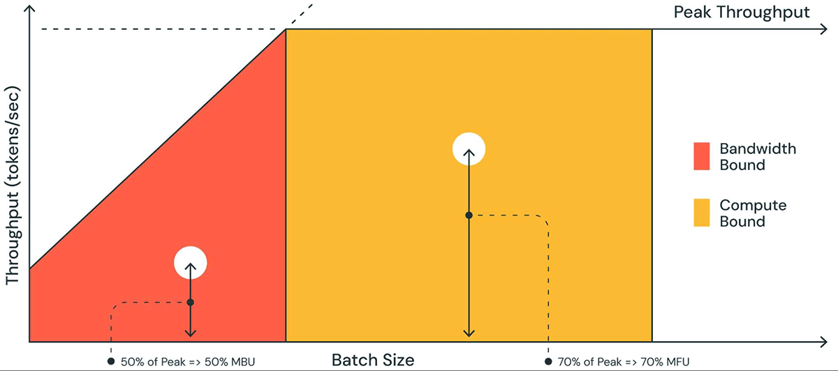
Figure 1 shows a pictorial representation of MBU in a plot similar to a roofline plot. The solid sloped line of the orange-shaded region shows the maximum possible throughput if memory bandwidth is fully saturated at 100%. However, in reality for low batch sizes (white dot), the observed performance is lower than maximum – how much lower is a measure of the MBU. For large batch sizes (yellow region), the system is compute bound, and the achieved throughput as a fraction of the peak possible throughput is measured as the Model Flops Utilization (MFU).
MBU and MFU determine how much more room is available to push the inference speed further on a given hardware setup. Figure 2 shows measured MBU for different degrees of tensor parallelism with our TensorRT-LLM-based inference server. Peak memory bandwidth utilization is attained when transferring large contiguous memory chunks. When smaller models like MPT-7B are distributed across multiple GPUs, we observe lower MBU as we are moving smaller memory chunks in each GPU.
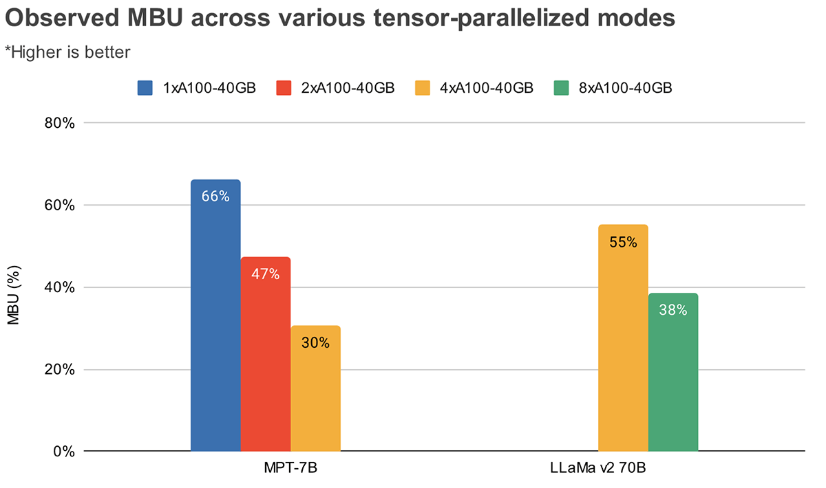
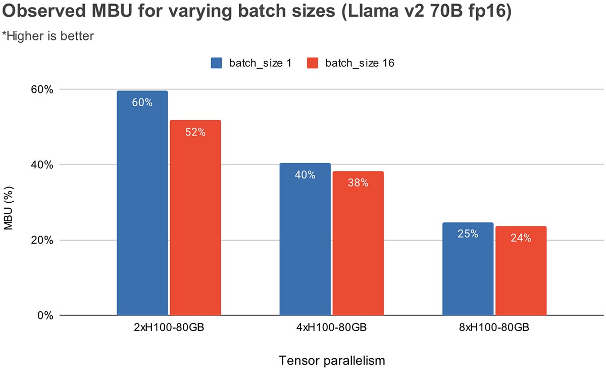
Figure 3 shows empirically observed MBU for different degrees of tensor parallelism and batch sizes on the NVIDIA H100 GPUs. MBU decreases as batch size increases. However, as we scale GPUs, the relative decrease in MBU is less significant. It is also worthy to note that picking hardware with greater memory bandwidth can boost performance with fewer GPUs. At batch size 1, we can achieve a higher MBU of 60% on 2xH100-80GBs as compared to 55% on 4xA100-40GB GPUs (Figure 2).
Benchmarking Results
Latency
We have measured time to first token (TTFT) and time per output token (TPOT) across different degrees of tensor parallelism for MPT-7B and Llama2-70B models. As input prompts lengthen, time to generate the first token starts to consume a substantial portion of total latency. Tensor parallelizing across multiple GPUs helps reduce this latency.
Unlike model training, scaling to more GPUs offers significant diminishing returns for inference latency. Eg. for Llama2-70B going from 4x to 8x GPUs only decreases latency by 0.7x at small batch sizes. One reason for this is that higher parallelism has lower MBU (as discussed earlier). Another reason is that tensor parallelism introduces communication overhead across a GPU node.
| Time to first token (ms) | ||||
|---|---|---|---|---|
| Model | 1xA100-40GB | 2xA100-40GB | 4xA100-40GB | 8xA100-40GB |
| MPT-7B | 46 (1x) | 34 (0.73x) | 26 (0.56x) | - |
| Llama2-70B | Doesn't fit | 154 (1x) | 114 (0.74x) | |
Table 1: Time to first token given input requests are 512 tokens length with batch size of 1. Larger models like Llama2 70B needs at least 4xA100-40B GPUs to fit in memory
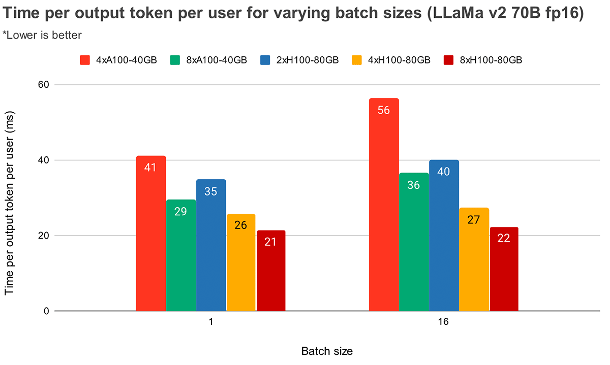
At larger batch sizes, higher tensor parallelism leads to a more significant relative decrease in token latency. Figure 4 shows how time per output token varies for MPT-7B. At batch size 1, going from 2x to 4x only reduces token latency by ~12%. At batch size 16, latency with 4x is 33% lower than with 2x. This goes in line with our earlier observation that the relative decrease in MBU is smaller at higher degrees of tensor parallelism for batch size 16 as compared to batch size 1.
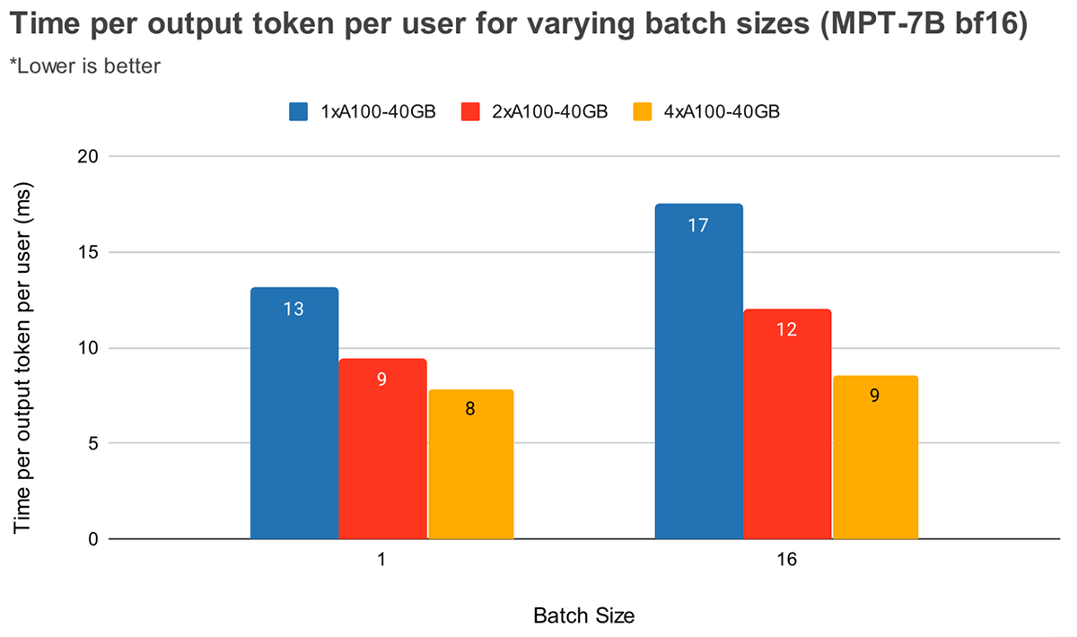
Figure 5 shows similar results for Llama2-70B, except the relative improvement between 4x and 8x is less pronounced. We also compare GPU scaling across two different hardware. Because H100-80GB has 2.15x GPU memory bandwidth as compared to A100-40GB, we can see that latency is 36% lower at batch size 1 and 52% lower at batch size 16 for 4x systems.
Throughput
We can trade off throughput and time per token by batching requests together. Grouping queries during GPU evaluation increases throughput compared to processing queries sequentially, but each query will take longer to complete (ignoring queueing effects).
There are a few common techniques for batching inference requests:
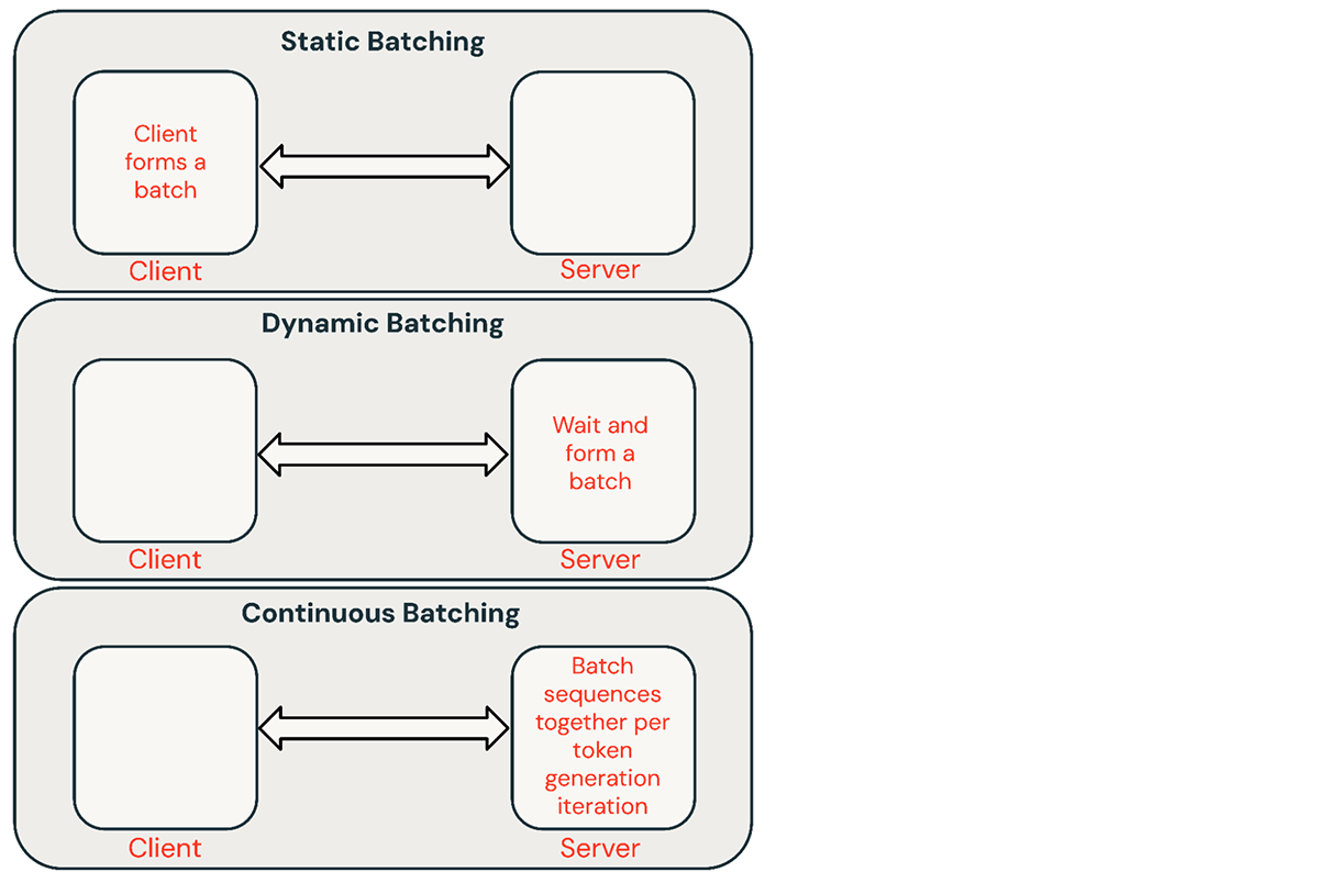
- Static batching: Client packs multiple prompts into requests and a response is returned after all sequences in the batch have been completed. Our inference servers support this but do not require it.
- Dynamic batching: Prompts are batched together on the fly inside the server. Typically, this method performs worse than static batching but can get close to optimal if responses are short or of uniform length. Does not work well when requests have different parameters.
- Continuous batching: The idea of batching requests together as they arrive was introduced in this excellent paper and is currently the SOTA method. Instead of waiting for all sequences in a batch to finish, it groups sequences together at the iteration level. It can achieve 10x-20x better throughput than dynamic batching.
Continuous batching is usually the best approach for shared services, but there are situations where the other two might be better. In low-QPS environments, dynamic batching can outperform continuous batching. It is sometimes easier to implement low-level GPU optimizations in a simpler batching framework. For offline batch inference workloads, static batching can avoid significant overhead and achieve better throughput.
Batch Size
How well batching works is highly dependent on the request stream. But we can get an upper bound on its performance by benchmarking static batching with uniform requests.
| Batch size | |||||||
|---|---|---|---|---|---|---|---|
| Hardware | 1 | 4 | 8 | 16 | 32 | 64 | 128 |
| 1 x A10 | 0.4 (1x) | 1.4 (3.5x) | 2.3 (6x) | 3.5 (9x) | OOM (Out of Memory) error | ||
| 2 x A10 | 0.8 | 2.5 | 4.0 | 7.0 | 8.0 | ||
| 1 x A100 | 0.9 (1x) | 3.2 (3.5x) | 5.3 (6x) | 8.0 (9x) | 10.5 (12x) | 12.5 (14x) | |
| 2 x A100 | 1.3 | 3.0 | 5.5 | 9.5 | 14.5 | 17.0 | 22.0 |
| 4 x A100 | 1.7 | 6.2 | 11.5 | 18.0 | 25.0 | 33.0 | 36.5 |
Table 2: Peak MPT-7B throughput (req/sec) with static batching and a FasterTransformers-based backend. Requests: 512 input and 64 output tokens. For larger inputs, the OOM boundary will be at smaller batch sizes.
Latency Trade-Off
Request latency increases with batch size. With one NVIDIA A100 GPU, for example, if we maximize throughput with a batch size of 64, latency increases by 4x while throughput increases by 14x. Shared inference services typically pick a balanced batch size. Users hosting their own models should decide the appropriate latency/throughput trade-off for their applications. In some applications, like chatbots, low latency for fast responses is the top priority. In other applications, like batched processing of unstructured PDFs, we might want to sacrifice the latency to process an individual document to process all of them fast in parallel.
Figure 7 shows the throughput vs latency curve for the 7B model. Each line on this curve is obtained by increasing the batch size from 1 to 256. This is useful in determining how large we can make the batch size, subject to different latency constraints. Recalling our roofline plot above, we find that these measurements are consistent with what we would expect. After a certain batch size, i.e., when we cross to the compute bound regime, every doubling of batch size just increases the latency without increasing throughput.
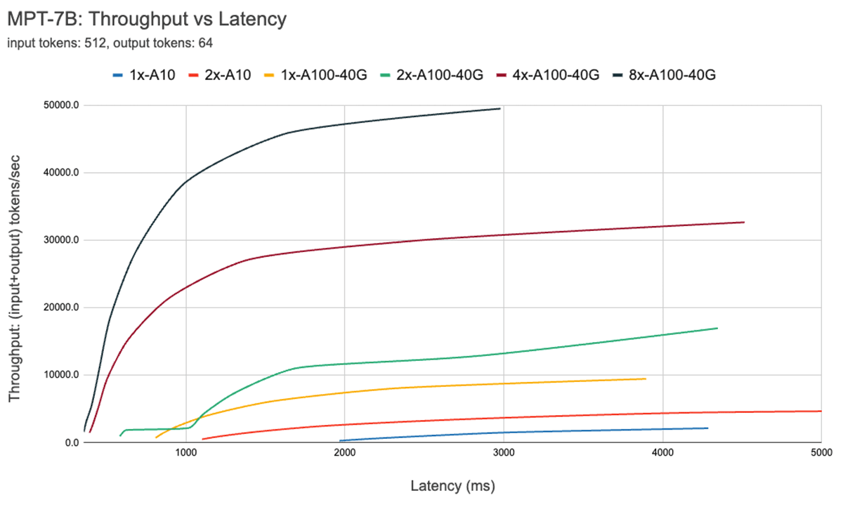
When using parallelism, it's important to understand low-level hardware details. For instance, not all 8xA100 instances are the same across different clouds. Some servers have high bandwidth connections between all GPUs, others pair GPUs and have lower bandwidth connections between pairs. This could introduce bottlenecks, causing real-world performance to deviate significantly from the curves above.
Optimization Case Study: Quantization
Quantization is a common technique used to reduce the hardware requirements for LLM inference. Reducing the precision of model weights and activations during inference can dramatically reduce hardware requirements. For instance, switching from 16-bit weights to 8-bit weights can halve the number of required GPUs in memory constrained environments (eg. Llama2-70B on A100s). Dropping down to 4-bit weights makes it possible to run inference on consumer hardware (eg. Llama2-70B on Macbooks).
In our experience, quantization should be implemented with caution. Naive quantization techniques can lead to a substantial degradation in model quality. The impact of quantization also varies across model architectures (eg. MPT vs Llama) and sizes. We will explore this in more detail in a future blog post.
When experimenting with techniques like quantization, we recommend using an LLM quality benchmark like the Mosaic Eval Gauntlet to evaluate the quality of the inference system, not just the quality of the model in isolation. Additionally, it's important to explore deeper systems optimizations. In particular, quantization can make KV caches much more efficient.
As mentioned previously, in autoregressive token generation, past Key/Values (KV) from the attention layers are cached instead of recomputing them at every step. The size of the KV cache varies based on the number of sequences processed at a time and the length of these sequences. Moreover, during each iteration of the next token generation, new KV items are added to the existing cache making it bigger as new tokens are generated. Therefore, effective KV cache memory management when adding these new values is critical for good inference performance. Llama2 models use a variant of attention called Grouped Query Attention (GQA). Please note that when the number of KV heads is 1, GQA is the same as Multi-Query-Attention (MQA). GQA helps with keeping the KV cache size down by sharing Keys/Values. The formula to calculate KV cache size is
batch_size * seqlen * (d_model/n_heads) * n_layers * 2 (K and V) * 2 (bytes per Float16) * n_kv_heads
Table 3 shows GQA KV cache size calculated at different batch sizes at a sequence length of 1024 tokens. The parameter size for Llama2 models, in comparison, is 140 GB (Float16) for the 70B model. Quantization of KV cache is another technique (in addition to GQA/MQA) to reduce the size of KV cache, and we are actively evaluating its impact on the generation quality.
| Batch Size | GQA KV cache memory (FP16) | GQA KV cache memory (Int8) |
|---|---|---|
| 1 | .312 GiB | .156 GiB |
| 16 | 5 GiB | 2.5 GiB |
| 32 | 10 GiB | 5 GiB |
| 64 | 20 GiB | 10 GiB |
Table 3: KV cache size for Llama-2-70B at a sequence length of 1024
As mentioned previously, token generation with LLMs at low batch sizes is a GPU memory bandwidth-bound problem, i.e. the speed of generation depends on how quickly model parameters can be moved from the GPU memory to on-chip caches. Converting model weights from FP16 (2 bytes) to INT8 (1 byte) or INT4 (0.5 byte) requires moving less data and thus speeds up token generation. However, quantization may negatively impact the model generation quality. We are currently evaluating the impact on model quality using Model Gauntlet and plan to publish a followup blog post on it soon.
Conclusions and Key Results
Each of the factors we've outlined above influences the way we build and deploy models. We use these results to make data-driven decisions that take into consideration the hardware type, the software stack, the model architecture, and typical usage patterns. Here are some recommendations drawn from our experience.
Identify your optimization target: Do you care about interactive performance? Maximizing throughput? Minimizing cost? There are predictable trade-offs here.
Pay attention to the components of latency: For interactive applications time-to-first-token drives how responsive your service will feel and time-per-output-token determines how fast it will feel.
Memory bandwidth is key: Generating the first token is typically compute-bound, while subsequent decoding is memory-bound operation. Because LLM inference often operates in memory-bound settings, MBU is a useful metric to optimize for and can be used to compare the efficiency of inference systems.
Batching is critical: Processing multiple requests concurrently is critical for achieving high throughput and for effectively utilizing expensive GPUs. For shared online services continuous batching is indispensable, whereas offline batch inference workloads can achieve high throughput with simpler batching techniques.
In depth optimizations: Standard inference optimization techniques are important (eg. operator fusion, weight quantization) for LLMs but it's important to explore deeper systems optimizations, especially those which improve memory utilization. One example is KV cache quantization.
Hardware configurations: The model type and expected workload should be used to decide deployment hardware. For instance, when scaling to multiple GPUs MBU falls much more rapidly for smaller models, such as MPT-7B, than it does for larger models, such as Llama2-70B. Performance also tends to scale sub-linearly with higher degrees of tensor parallelism. That said, a high degree of tensor parallelism might still make sense for smaller models if traffic is high or if users are willing to pay a premium for extra low latency.
Data Driven Decisions: Understanding the theory is important, but we recommend always measuring end-to-end server performance. There are many reasons an inference deployment can perform worse than expected. MBU could be unexpectedly low because of software inefficiencies. Or differences in hardware between cloud providers could lead to surprises (we have observed a 2x latency difference between 8xA100 servers from two cloud providers).
To get started with LLM inference, try out Databricks Model Serving. Check out the documentation to learn more.
Get the latest posts in your inbox
Subscribe to our blog and get the latest posts delivered to your inbox.