Part Level Demand Forecasting at Scale
Predict the moving target of supply and demand to streamline your manufacturing operations
by Max Köhler, Pawarit Laosunthara, Bryan Smith and Bala Amavasai

Check out our Part Level Demand Forecasting Accelerator for more details and to download the notebooks.
Demand forecasting is a critical business process for manufacturing and supply chains. A survey by Deloitte found that 40% of CFOs surveyed indicated that supply chain shortages or delays increased their bottom line costs by 5% or more. 60% of those surveyed indicated that sales had reduced due to the current disruptions. McKinsey estimates that over the next 10 years, supply chain disruptions can cost close to half (~45%) of a year's worth of profits for companies. A disruption lasting just 30 days or less could equal losses of 3-5% of EBITDA. Having accurate and up-to-date forecasts is vital to plan the scaling of manufacturing operations, ensure sufficient inventory and guarantee customer fulfillment.
The challenges of demand forecasting include ensuring the right granularity, timeliness, and fidelity of forecasts. Due to limitations in computing capability and the lack of know-how, forecasting is often performed at an aggregated level, reducing fidelity.
In this blog, we demonstrate how our Solution Accelerator for Part Level Demand Forecasting helps your organization to forecast at the part level, rather than at the aggregate level using the Databricks Lakehouse Platform. Part-level demand forecasting is especially important in discrete manufacturing where manufacturers are at the mercy of their supply chain. This is due to the fact that constituent parts of a discrete manufactured product (e.g. cars) are dependent on components provided by third-party original equipment manufacturers (OEMs).
New global challenges require granular forecasting
In recent years, manufacturers have been investing heavily in quantitative-based forecasting that is driven by historical data and powered using either statistical or machine learning techniques.
Demand forecasting has proven to be very successful in pre-pandemic years. The demand series for products had relatively low volatility and the likelihood of material shortages was relatively small. Therefore, manufacturers simply interpreted the number of shipped products as the "true" demand and used highly sophisticated statistical models to extrapolate into the future. This provided:
- Improved sales planning
- Highly optimized safety stock that allowed maximizing turn-rates and service-delivery performance
- An optimized production planning by tracing back production outputs to raw material level using the bill of materials (BoM)
However, since the pandemic, demand has seen unprecedented volatility and fluctuations. Production output and actual demand often fall out of sync, leading to under-planning and guess-work-based approaches to increase safety stock. Traditional demand planning approaches are incompatible with current operating conditions, costing the industry billions of dollars in lost revenues and reputational damage to brands unable to deliver products on time or at all.
At the onset of the pandemic, demand dropped significantly in the early days of stay-at-home measures. Expecting a muted outlook to persist, a number of suppliers under-planned production capacity based on inaccurate demand forecasts. Inaccurate and outdated forecasts rendered collaboration with the deeper tier suppliers ineffective, making the problem worse. The V-shaped recovery resulted in a surge of orders and the bottlenecks created by traditional demand forecasting approaches and ineffective planning kicked off a multi-tier supply crisis impacting overall industry output.
A perfect example can be found in the chip crisis, where a shortage in semiconductors has had ripple effects on downstream industries. In addition to demand shocks, automotive manufacturers and suppliers have had to contend with supply chain pressures for semiconductors.
Several exogenous factors (trade wars, weather, and geopolitical conflict) have made forecasting demand and production challenging. The trade war between China and the United States imposed restrictions on China's largest chip manufacturer. The Texas ice storm of 2021 resulted in a power crisis that forced the closure of several computer-chip facilities; Texas is the center of semiconductor manufacturing in the US. Taiwan experienced a severe drought which further reduced the supply. Two Japanese plants caught fire, one as a result of an earthquake (source).
Could statistical demand forecasting have predicted the aforementioned 'force majeure' events far before they happened? Certainly not. But if these forecasts are done at more regular intervals, rather than monthly or quarterly, the fidelity of subsequent forecasts can drastically improve. This is due to the fact that forecasting algorithms work far better on shorter forecast horizons and will be able to more accurately track a disruption as it happens. Using such forecasts to drive more effective production planning and supplier collaboration will ultimately yield higher service levels and profitability for manufacturers.
The Databricks Lakehouse Platform for part-level forecasting
Databricks offers a complete platform to build large-scale forecasting solutions to help manufacturers navigate these challenges. These include:
- Collaborative notebooks (in Python, R, SQL, and Scala) that can be used to explore, enrich, and visualize data from multiple sources while accommodating business knowledge and domain expertise
- Fine-grained modeling and forecasting per item (e.g. product, SKU, or part) that can be parallelized, scaling to thousands, if not hundreds of thousands of items
- Tracking experiments using MLFlow ensures reproducibility, traceable performance metrics, and easy re-use
Building the solution
To showcase the benefits of using Databricks and our Part Level Forecasting Solution Accelerator, we will leverage a simulated data set and assume the role of a tier one automotive manufacturer producing advanced driver assistance systems. We will then proceed in three steps:
- Part level (or fine-grained) demand forecasting
- Derivation of raw material demand
- Manage shortages
Our forecasting algorithm of choice for this use case is SARIMAX. SARIMAX belongs to the ARIMA family of models but also accounts for seasonality in the data as well as external variables. We choose to use the SARIMAX algorithm provided by statsmodels. We also use hyperopt to perform hyperparameter tuning from within a Pandas UDF (user-defined function).
Forecasting demand
We first read our input dataset into a Spark DataFrame. For discoverability and governance best practices, the input data can be registered as either a managed or external table in Unity Catalog.
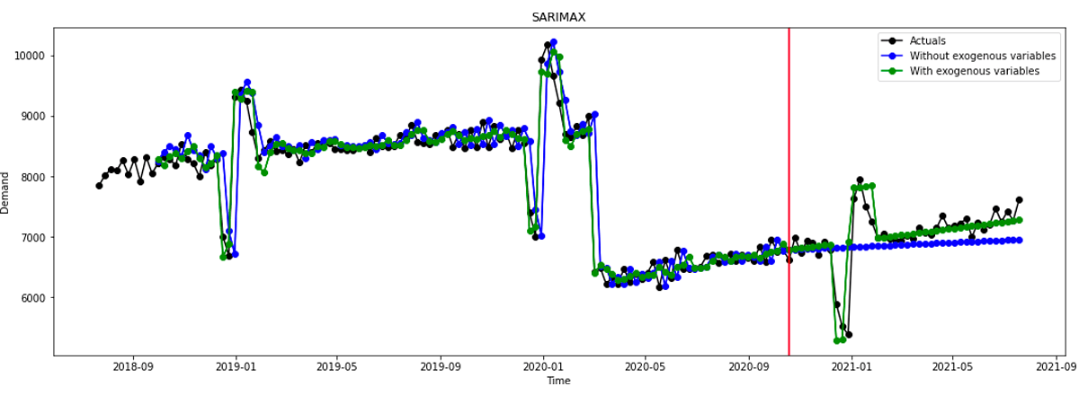
As a baseline, we can initially fit a SARIMAX model of order p=1, d=2, q=1 with exogenous variables for the COVID-19 outbreak as well as the Christmas/New Year period as follows:
The forecast is shown in Figure 1. The red vertical line indicates the start of the forecast horizon. The green line shows the forecast accounting for exogenous variables (in this case, the Christmas/New Year period in January 2021) vs the line in blue which does not account for this external factor.
Hyperparameter optimization
In the previous section, we manually selected values for our parameters p, d, and q. However, we can more efficiently automate hyperparameter optimization using Hyperopt:
where the hyperopt_params above are sampled from the search space defined below:
Leveraging applyInPandas() to scale across thousands of series
For computationally intensive problems, such as building forecasts for tens or hundreds of thousands of SKUs, a big data processing engine such as Apache Spark on Databricks is typically used to distribute computation across multiple nodes. Individual worker nodes within the Databricks cluster can train multiple models in parallel, thus reducing time-to-insight while also simplifying infrastructure management thanks to elastic, scalable compute as well as intuitive Workflows orchestration.
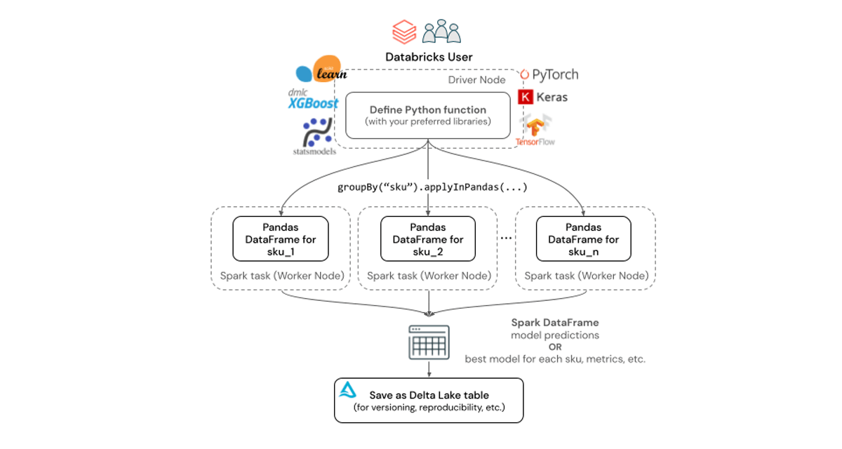
In this example, we can use pandas function APIs (such as applyInPandas), to parallelize and speed-up model training using a Spark cluster. Conceptually, we can group the data by Product & SKU, then train a model for each one of these groups. However, to maximize parallelism, we first need to ensure that each group is allocated its own Spark task. We achieve this by disabling Adaptive Query Execution (AQE) just for this step and partitioning our input Spark DataFrame as follows:
In the code segment above, build_tune_and_score_model is the primary function that not only fits the SARIMAX model, but also incorporates Hyperopt for hyperparameter tuning. The groupBy() + applyInPandas() pattern allows us to split our large Spark DataFrame into independent Pandas DataFrames by each unique Product & SKU combination. Users can then simply drop in their existing Python functions (which often involve Pandas DataFrames and their Python libraries of choice) and then leave Databricks to handle parallelization and autoscaling.
Mapping per-SKU demand to raw materials
In the last section, we discuss the advantages of using parallel processing in Databricks to forecast the demand for thousands of SKUs. However, knowing the approximate demand for each SKU at some future point alone does not suffice to achieve operational efficiency gains as long as no action is triggered from this knowledge. Manufacturers typically do not simply place an order for products like a retailer. Instead, they need to produce them.
Once the demand is forecasted, manufacturers need to purchase raw materials from deeper-tier suppliers and initiate production planning. This notebook shows how to translate future demand into raw materials. More precisely, we will do a bill of material (BoM) resolution to map the forecasted demand for each SKU to the appropriate demand of raw materials that are needed to produce the finished goods that are mapped to the SKU. The BoM data is typically stored within SAP ERP.
BoM resolution and traversing the manufacturing value chain backward
Let us consider a typical BoM as shown in figure 2. The figure represents a building plan for a finished product and therefore consists of several intermediate products, raw materials, and necessary quantities.
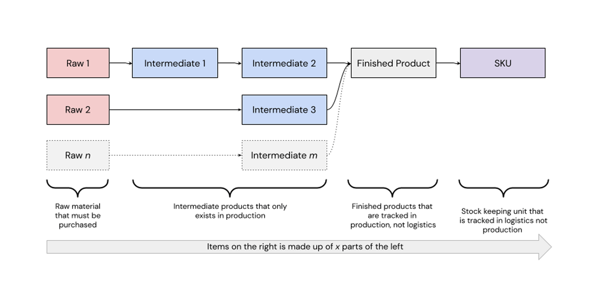
In reality, a BoM has many more and a previously unknown number of steps. Needless to say that this also means that there are many more raw materials and intermediate products.
The figure above assumes that the final product is mapped to one SKU. This information would not be part of a typical BoM as it is mainly relevant in production systems, whereas an SKU is rather a logistics term. We assume that a look-up table exists that maps each finished product to its SKU. The above BoM is then a result of artificially adding another step with quantity 1.
We now translate the manufacturing terms into terms that are used in graph theory: Each assembly step is an edge; the raw materials, intermediate products, the finished product, and the SKU are vertices. The edge dataset of this graph is the BoM and vertices can be easily derived from the edges.
Let's first create the graph:
The goal is to map the forecasted demand values for each SKU to quantities of the raw materials (the input of the production line) that are needed to produce the associated finished product (the output of the production line). To this end, we need a table that lists for each SKU demand at each time point all raw materials that are needed for production (ideally also a just-in-time view to reducing warehouse costs). We do this in two steps:
- Derive the SKU for each raw material.
- Derive the product of all quantities of all succeeding assembly steps (=edges) from a raw material point of view.
Functions that apply the concept of aggregated messaging (see the GraphX programming guide) are implemented in the solution accelerator as follows:
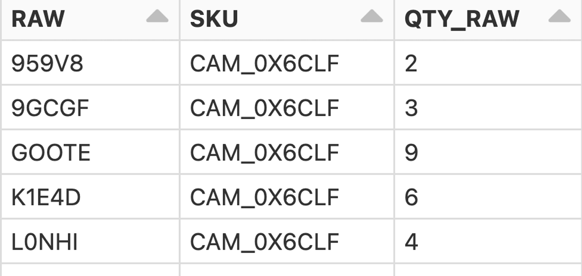
Step 1:
Result:

Step 2:
Result:
Deducing future raw material demand from SKU forecasts
We start with reading the forecasted demand and creating the edge and vertices dataset to derive the graph. Note that the SKU is added to the BoM by artificially adding another edge with quantity 1 for each SKU (=parent) and finished product (=child) combination.
We now apply the two steps mentioned previously:
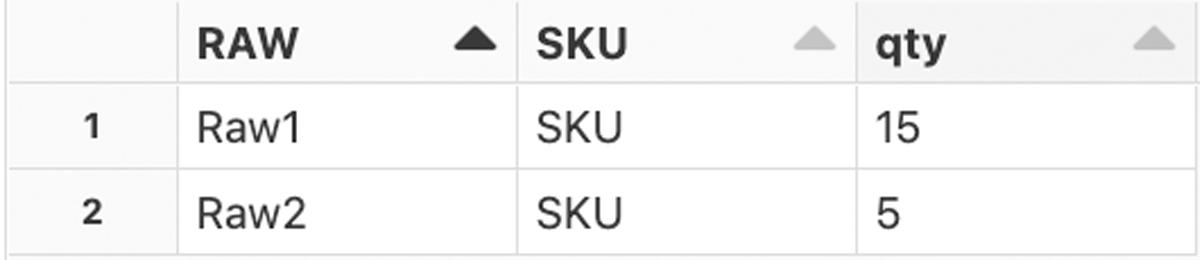
Joining the two tables yields the desired aggregated BoM:
We now see row-wise which and how many of the raw materials enter each SKU. Deriving the demand for the raw materials is now straightforward since we have forecasts at the SKU level.
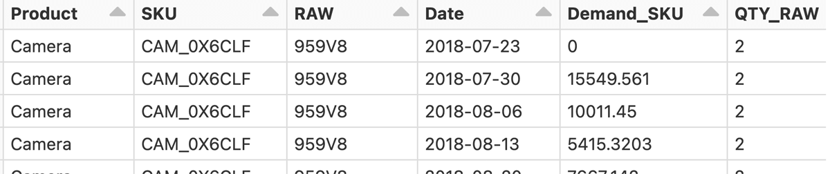
This table shows the raw materials and their quantities at each time point (and future ones based on the SKU forecast). This alone facilitates production and purchasing planning.
Managing material shortages
Communication with suppliers would normally occur using modern ERP platforms with the ability to share data using EDI (electronic data exchange) standards. However, despite the availability of modern platforms, many suppliers still do resort to semi-structured and unstructured means of communication, e.g. paper, e-mail, and phone. The ability to store, process, and recall this information using the Lakehouse architecture is vital.
After checking with the supplier how much raw material can actually be delivered we can now traverse the manufacturing value chain forwards to find out how many SKUs can actually be shipped to the customer. If one raw material is the bottleneck for producing a specific SKU, orders of the other raw materials for that SKU can be adjusted accordingly to save storage costs.
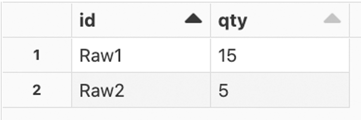
In our specific case, the following three raw materials have shortages.
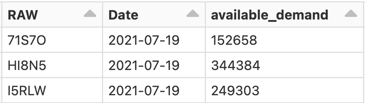
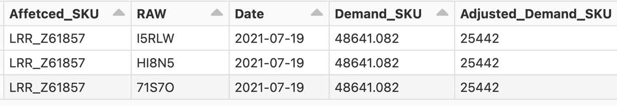
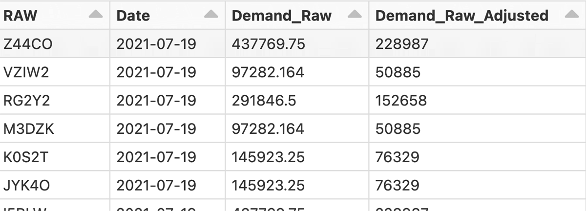
We can now check if the forecasted demands exceed the available demands and report on the affected SKUs. This serves to notify downstream customers in advance. On the other hand, if the finished product for an SKU cannot be delivered in full, other raw materials that serve as input to that product are overplanned. We correct for the overplanning to decrease storage costs. The associated Python code is lengthy due to data wrangling, but it is straightforward as shown in the attached notebooks. The results are mainly a table with the affected SKUs
A table to adjust for the overplanning of the raw materials is also given:
Get started with part-level forecasting
As the current supply chain challenges continue to cause global bottlenecks, it is imperative that manufacturers are able to navigate through the climate of persistent uncertainty.
Try our solution accelerator to build part level demand forecasting at your organization, and improve the quality of your overall forecasts by doing it at a much finer grain.
Get the latest posts in your inbox
Subscribe to our blog and get the latest posts delivered to your inbox.