eBook
Comprehensive Guide to Optimize Databricks, Spark and Delta Lake Workloads

Authors:
Himanshu Arora, Senior Resident Solutions Architect
Prashanth Babu Velanati Venkata, Lead Product Specialist
Introduction
This document aims to compile most (if not all) of the essential Databricks, Apache Spark™, and Delta Lake best practices and optimization techniques in one place. All data engineers and data architects can use it as a guide when designing and developing optimized and cost-effective and efficient data pipelines. Costs should not be treated as an afterthought but as one of the most important nonfunctional requirements right at the inception of the project. As a result, all of the best practices discussed in this book should be considered throughout the development and productionization of data pipelines. This book is divided into several sections, each focusing on a particular problem statement and deep diving into providing all the possible solutions for it.
Delta Lake — The Lakehouse Format
Delta Lake is an open format storage layer that delivers reliability, security and performance on your data lake. It enables building a Lakehouse architecture with compute engines including Spark, PrestoDB, Flink, Trino, and Hive, and APIs for Python, SQL, Scala, Java, Rust, and Ruby. It has many benefits over other open formats like Parquet, Avro, ORC, etc. — for example:
- Delta is a protocol to guarantee ACID transactions, high performance and a ton of other features on top of the open source Parquet format. Delta is open source and the complete protocol can be found here.
- Delta Lake supports ACID transactions and unifies batch and streaming paradigms, simplifying delete/insert/update transactions on incremental data
- Delta allows you to time travel and to read a point-in-time snapshot version of the table
- Delta also comes with many performance enhancements around efficient data layout, indexation, data skipping and caching, etc.
Therefore, it is highly recommended to use Delta as the default data lake storage format to reap all the benefits. On Databricks DBR 8.x and above, Delta Lake is the default format.
Underlying Data Layout
Underneath the hood of a Delta table are Parquet files that store the data. It also contains a subdirectory named _delta_log that stores the Delta transaction logs right next to the Parquet files. The size of these Parquet files is really crucial for query performance.
The tiny files problem is a well-known problem in the big data world. When a table has too many underlying tiny files, read latency suffers as a result of the time spent for just opening and closing those tiny files.
To avoid this problem, it’s best to have a file size between 16MB and 1GB, which is configurable on a case-by-case basis based on the workload and the specific use case.
If you are using Databricks Runtime 11.3 and above to create managed Delta tables cataloged in Unity Catalog (Databricks’ data catalog), you don’t need to worry about optimizing the underlying file sizes or configuring a target file size for your Delta tables because Databricks will carry out this task automatically in the background as part of the auto-tuning capability. In the future, this will also be available for external tables.
For the remaining cases, you would need to manually compact files together using specific Spark jobs to obtain the appropriate file size, but this isn’t necessary with Delta tables because they come with out-of-the-box bin packing (compaction) features. In Delta, bin packing can be accomplished in two ways, as detailed below:
1. Optimize & Z-order
OPTIMIZE compacts the files to get a file size of up to 1GB, which is configurable. This command basically attempts to size the files to the size that you have configured (or 1GB by default if not configured). You can also combine the OPTIMIZE command with the ZORDER, which physically sorts or co-locates data by chosen column(s).
![]()
- Always choose high cardinality columns (for example:
customer_idin an orders table) for Z-ordering. Date columns are usually low cardinality columns, so they should not be used for Z-order — they are a better fit as the partitioning columns (but you don’t always have to partition the tables; please refer to the Partitioning section below for more details). For Z-order, choose the columns that are most frequently used in filter clauses or as join keys in the downstream queries. - Never use more than 4 columns since too many columns will degrade Z-ordering effectiveness
- Always run OPTIMIZE command on a separate job cluster and not as part of the job itself; otherwise, it might impact the corresponding job’s SLA
- Compute-optimized instance family is recommended for the OPTIMIZE command as it’s a compute-intensive operation
- OPTIMIZE (with or without ZORDER) should be done on a regular basis, such as once a day (or weekly or as per your requirements), to maintain a good file layout for better downstream query performance
2. Auto optimize
Auto optimize, as the name suggests, automatically compacts small files during individual writes to a Delta table, and by default, it tries to achieve a file size of 128MB. It comes with two features:
1. Optimize Write
Optimize Write dynamically optimizes Apache Spark partition sizes based on the actual data, and attempts to write out 128MB files for each table partition. It’s done inside the same Spark job.
2. Auto Compact
Following the completion of the Spark job, Auto Compact launches a new job to see if it can further compress files to attain a 128MB file size.
![]()
- Always enable optimizeWrite table property if you are not already leveraging the manual OPTIMIZE (with or without ZORDER) command to get a decent file size. Keep in mind that optimized writes require the shuffling of data according to the partitioning structure of the target table. This shuffle naturally incurs additional cost. However, the throughput gains during the write may pay off the cost of the shuffle. If not, the throughput gains when querying the data should still make this feature worthwhile.
- If your job isn’t strictly SLA bound, then in that case you can also enable autoCompact table property to further take advantage of Delta bin packing
3. Partitioning
Partitioning can speed up your queries if you provide the partition column(s) as filters or join on partition column(s) or aggregate on partition column(s) or merge on partition column(s), as it will help Spark to skip a lot of unnecessary data partition (i.e., subfolders) during scan time.
![]()
- Databricks recommends not to partition tables under 1TB in size and let ingestion time clustering automatically take effect. This feature will cluster the data based on the order the data was ingested by default for all tables.
- You can partition by a column if you expect data in each partition to be at least 1GB
- Always choose a low cardinality column — for example, year, date — as a partition column
- You can also take advantage of Delta’s generated columns feature while choosing the partition column. Generated columns are a special type of column whose values are automatically generated based on a user-specified function over other columns in the Delta table.
4. File size tuning
In cases where the default file size targeted by Auto-optimize (128MB) or Optimize (1GB) isn’t working for you, you can fine-tune it as per your requirement. You can set the target file size by using delta.targetFileSize table property and then Auto-optimize and Optimize will binpack to achieve the specified size instead.
You can also delegate this task to Databricks if you don’t want to manually set the target file size by turning on the delta.tuneFileSizesForRewrites table property. When this property is set to true, Databricks will automatically tune the file sizes based on workloads. For example, if you do a lot of merges on the Delta table, then the files will automatically be tuned to much smaller sizes than 1GB to accelerate the merge operation.

Data Shuffling — Why It Happens and How to Control It
Data shuffle occurs as a result of wide transformations such as joins, aggregations and window operations, among others. It is an expensive process since it sends data over the network between worker nodes. We may use a few optimization approaches to either eliminate or improve the efficiency and speed of shuffles.
1. Broadcast hash join
To entirely avoid data shuffling, broadcast one of the two tables or DataFrames (the smaller one) that are being joined together. The table is broadcast by the driver, who copies it to all worker nodes.
When executing joins, Spark automatically broadcasts tables less than 10MB; however, we may adjust this threshold to broadcast even larger tables, as demonstrated below:
When you know that some of the tables in your query are small tables, you can tell Spark to broadcast them explicitly using hints, which is a recommended option.
Spark 3.0 and above comes with AQE (Adaptive Query Execution), which can also convert the sort-merge join into broadcast hash join (BHJ) when the runtime statistics of any join side is smaller than the adaptive broadcast hash join threshold, which is 30MB by default. You can also increase this threshold by changing the following configuration:
![]()
- Note that broadcast hash join is not supported for a full outer join. For the right outer join, only the left-side table can be broadcast, and for other left joins only the right-side table can be broadcast.
If you’re running a driver with a lot of memory (32GB+), you can safely raise the broadcast thresholds to something like 200MB
- Always explicitly broadcast smaller tables using hints or PySpark broadcast function
- Why do we need to explicitly broadcast smaller tables if AQE can automatically broadcast smaller tables for us? The reason for this is that AQE optimizes queries while they are being executed.
- Spark needs to shuffle the data on both sides and then only AQE can alter the physical plan based on the statistics of the shuffle stage and convert to broadcast join
- Therefore, if you explicitly broadcast smaller tables using hints, it skips the shuffle altogether and your job will not need to wait for AQE’s intervention to optimize the plan
- Never broadcast a table bigger than 1GB because broadcast happens via the driver and a 1GB+ table will either cause OOM on the driver or make the drive unresponsive due to large GC pauses
- Please take note that the size of a table in disk and memory will never be the same. Delta tables are backed by Parquet files, which can have varying levels of compression depending on the data. And Spark might broadcast them based on their size in the disk — however, they might actually be really big (even more than 8GB) in memory after the decompression and conversion from column to row format. Spark has a hard limit of 8GB on the table size it can broadcast. As a result, your job may fail with an exception in this circumstance. In this case, the solution is to either disable broadcasting by setting
spark.sql.autoBroadcastJoinThresholdto -1 and do the explicit broadcast using hints (or the PySpark broadcast function) of the tables that are really small in the disk as well as in memory, or set thespark.sql.autoBroadcastJoinThresholdto smaller values like 100MB or 50MB instead of setting the threshold to -1. - The driver can only collect up to 1GB of data in memory at any given time, and anything more than that will trigger an error in the driver, causing the job to fail. However, since we want to broadcast tables larger than 10MB, we risk running into this problem. This problem can be solved by increasing the value of the following driver configuration.
- Please keep in mind that because this is a driver setting; it cannot be altered once the cluster is launched. Therefore, it should be set under the cluster’s advanced options as a Spark config. Setting this parameter to 8GB for a driver with >32GB memory seems to work fine in most circumstances. In certain cases where the broadcast hash join is going to broadcast a very large table, setting this value to 16GB would also make sense.
In Photon, we have the executor-side broadcast. So, you don’t have to change the following driver configuration if you use a Databricks Runtime (DBR) with Photon.
2. Shuffle hash join over sort-merge join
In most cases Spark chooses sort-merge join (SMJ) when it can’t broadcast tables. Sort-merge joins are the most expensive ones. Shuffle-hash join (SHJ) has been found to be faster in some circumstances (but not all) than sort-merge since it does not require an extra sorting step like SMJ. There is a setting that allows you to advise Spark that you would prefer SHJ over SMJ, and with that Spark will try to use SHJ instead of SMJ wherever possible. Please note that this does not mean that Spark will always choose SHJ over SMJ. We are simply defining your preference for this option.
Databricks Photon engine also replaces sort-merge join with shuffle hash join to boost the query performance.
![]()
- Setting the
preferSortMergeJoinconfig option to false for each job is not necessary. For the first execution of a concerned job, you can leave this value to default (which is true). - If the job in question performs a lot of joins, involving a lot of data shuffling and making it difficult to meet the desired SLA, then you can use this option and change the
preferSortMergeJoinvalue to false
3. Leverage cost-based optimizer (CBO)
Spark SQL can use a Cost-based optimizer (CBO) to improve query plans. This is especially useful for queries with multiple joins. The CBO is enabled by default. You disable the CBO by changing the following configuration:
For CBO to work, it is critical to collect table and column statistics and keep them up to date. Based on the stats, CBO chooses the most economical join strategy. So you will have to run the following SQL command on the tables to compute stats. The stats will be stored in the Hive metastore.
Join reorder
For faster query execution CBO can also use the stats calculated by ANALYZE TABLE command to find the optimal order in which the tables should be joined (for instance, joining smaller tables first would significantly improve the performance). Join reordering works only for INNER and CROSS joins. To leverage this feature, set the following configurations:
![]()
- To properly leverage CBO optimizations, ANALYZE TABLE command needs to be executed regularly (preferably once per day or when data has mutated by more than 10%, whichever happens first)
- When Delta tables are recreated or overwritten on a daily basis, the ANALYZE TABLE command should be executed immediately after the table is overwritten as part of the same job or pipeline. This will have an impact on your pipeline’s overall SLA. As a result, in cases like this, there is a trade-off between better downstream performance and the current job’s execution time. If you don’t want CBO optimization to affect the current job’s SLA, you can turn it off.
- Never run ANALYZE TABLE command as part of your job. It should be run as a separate job on a separate job cluster. For example, it can be run inside the same nightly notebook running commands like Optimize, Z-order and Vacuum.
- Leverage join reorder where a lot of inner-joins and/or cross-joins are being performed in a single query
- Spark’s Adaptive Query Execution (AQE), which changes the query plan on the fly during runtime to a better one, also takes advantage of the statistics calculated by ANALYZE TABLE command. Therefore, it’s recommended to run ANALYZE TABLE command regularly to keep the table statistics updated.

Data Spilling — Why It Happens and How to Get Rid of It
The default setting for the number of Spark SQL shuffle partitions (i.e., the number of CPU cores used to perform wide transformations such as joins, aggregations and so on) is 200, which isn’t always the best value. As a result, each Spark task (or CPU core) is given a large amount of data to process, and if the memory available to each core is insufficient to fit all of that data, some of it is spilled to disk. Spilling to disk is a costly operation, as it involves data serialization, de-serialization, reading and writing to disk, etc. Spilling needs to be avoided at all costs and in doing so, we must tune the number of shuffle partitions. There are a couple of ways to tune the number of Spark SQL shuffle partitions as discussed below.
1. AQE auto-tuning
Spark AQE has a feature called autoOptimizeShuffle (AOS), which can automatically find the right number of shuffle partitions. Set the following configuration to enable auto-tuning:
Caveat: unusually high compression
There are certain limitations to AOS. AOS may not be able to estimate the correct number of shuffle partitions in some circumstances where source tables have an unusually high compression ratio (20x to 40x).
There are two ways you can identify the highly compressed tables:
1. Spark UI SQL DAG
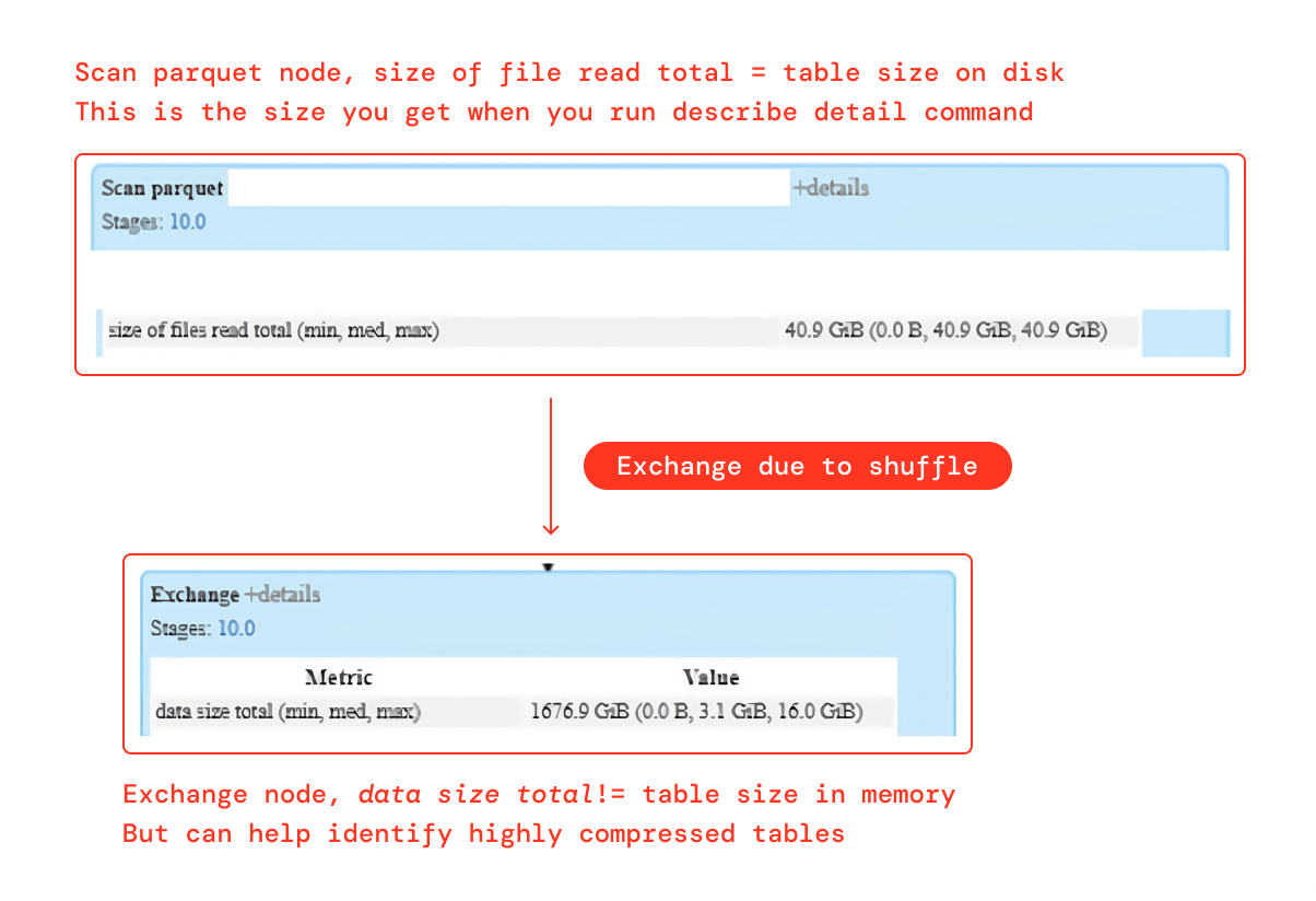
Although “data size total” metrics in the Exchange node don’t provide the exact size of a table in memory, it can definitely help identify the highly compressed tables. Scan Parquet node provides the precise size of a table in the disk. The Exchange node data size in the aforementioned case is 40x larger than the size on the disk, indicating that the table is probably heavily compressed on the disk.
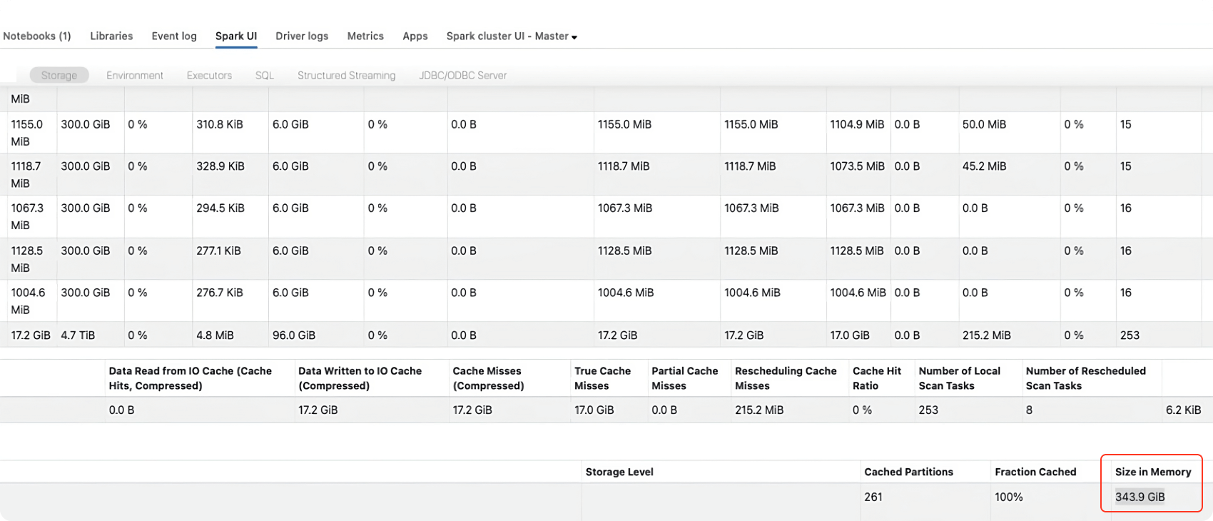
2. Cache the table
A table can be cached in memory to figure out its actual size in memory. Here’s how to go about it:
Refer to the storage tab of Spark UI to find the size of the table in memory after the command above has been completed:
Solution: To counter this effect, reduce the value of the per partition size used by AQE to determine the initial shuffle partition number (default 128MB) as follows:
After lowering the preshufflePartitionSizeInBytes value to 16MB, if AOS is still calculating the incorrect number of partitions and you are still experiencing large data spills, you should further lower the preshufflePartitionSizeInBytes value to 8MB. If this still doesn’t resolve your spill issue, it is best to disable AOS and manually tune the number of shuffle partitions as explained in the next section.
2. Manually fine-tune
To manually fine-tune the number of shuffle partitions we need:
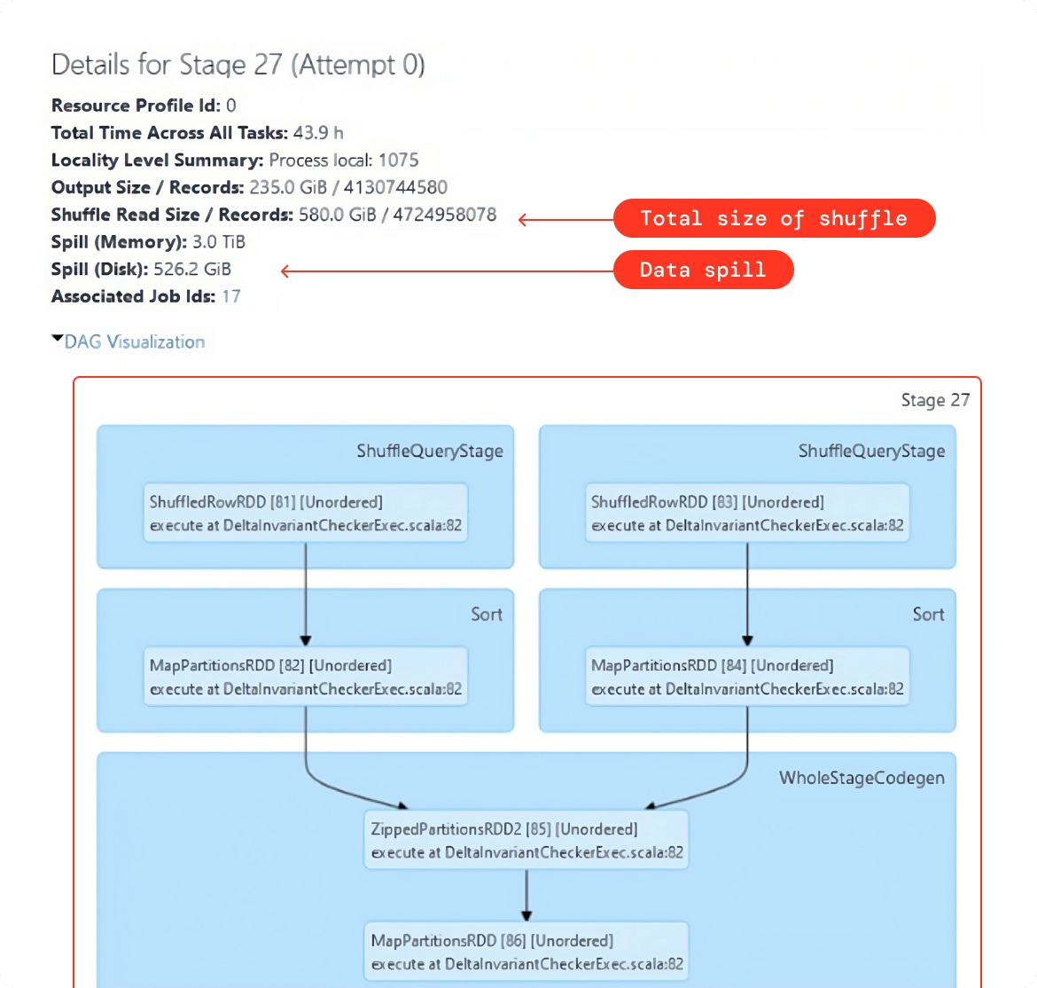
- The total amount of shuffled data. To do so, run the Spark query once, and then use the Spark UI to retrieve this value, as demonstrated in the example below:
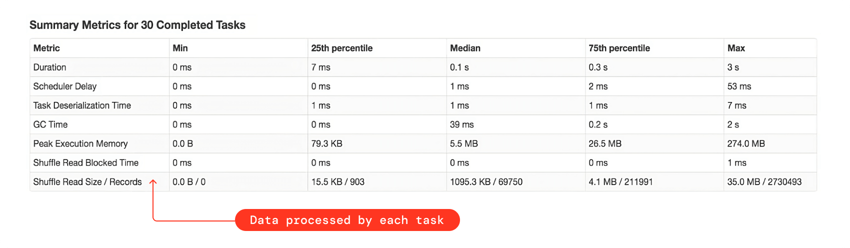
- As a rule of thumb, we need to make sure that after tuning the number of shuffle partitions, each task should approximately be processing 128MB to 200MB of data. You can see this value in the summary metrics for the shuffle stage in Spark UI, as shown in the example below:
So here is the formula to compute the right number of shuffle partitions:
![]()
- The optimal size of data to be processed per task should be 128MB approximately. It works well in most cases. It might not work if there is some sort of data explosion happening in your query. You might need to choose a smaller value in that case. We will have a section on data explosion later in this document.
If you are neither using auto-tune (AOS) nor manually fine-tuning the shuffle partitions, then as a rule of thumb set this to twice, or better thrice, the number of total worker CPU cores
- Because there may be multiple Spark SQL queries in a single notebook, fine-tuning the number of shuffle partitions for each query is a time-consuming task. So, our advice is to fine-tune it for the largest query with the greatest number for the total amount of data being shuffled for a shuffle stage and then set that value once for the entire notebook.
- If there is skewness in data, then fine-tuning the shuffle partitions will not help with data spills. In that case, you should first get rid of the data skew. Please refer to the next section on data skew for more details.

Data Skewness — Identification and Remediation
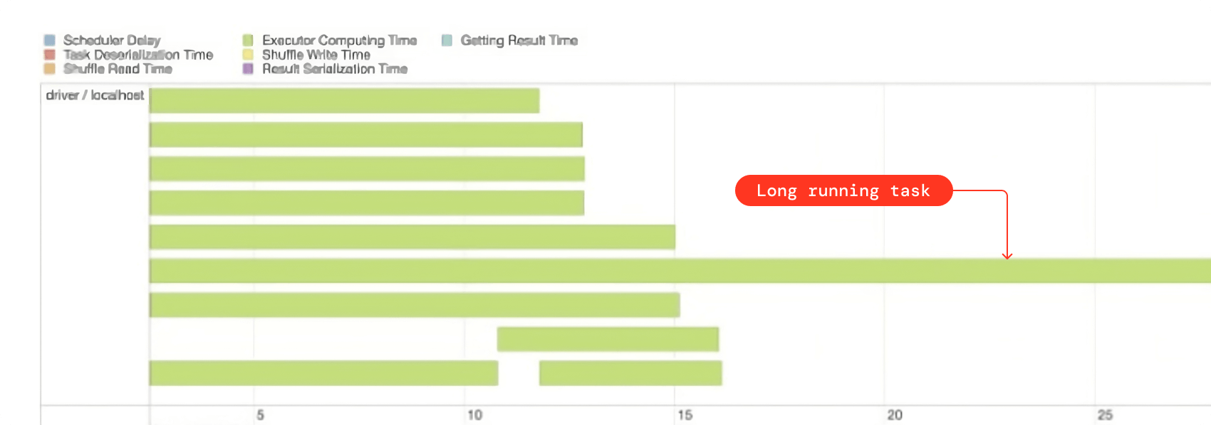
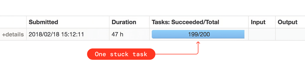
Data skew is the situation where only a few CPU cores wind up processing a huge amount of data due to uneven data distribution. For example, when you join or aggregate using the columns(s) around which data is not uniformly distributed, then you will end up with a skewed shuffle stage that will take a lot of time to finish (might actually fail as well after several attempts).
Identification of skew
- If all the Spark tasks for the shuffle stage are finished and just one or two of them are hanging for a long time, that’s an indication of skew. You can also get this information from Spark UI.
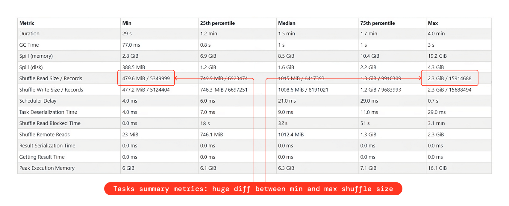
- In the tasks summary metrics, if you see a huge difference between the min and max shuffle read size, that’s also an indication of data skewness
- Even after fine-tuning the number of shuffle partitions, if there are a lot of data spills, then this might actually be because of skewness
- Lastly, you can just simply count the number of rows while grouping by join or aggregation columns. If there is an enormous disparity between the row counts, then it’s a definite skew.
Skew remediation
- Filter skewed values
If it’s possible to filter out the values around which there is a skew, then that will easily solve the issue. If you join using a column with a lot of null values, for example, you’ll have data skew. In this scenario, filtering out the null values will resolve the issue. Skew hints
In the case where you are able to identify the table, the column, and preferably also the values that are causing data skew, then you can explicitly tell Spark about it using skew hints so that Spark can try to resolve it for you.AQE skew optimization
Spark 3.0+’s AQE can also dynamically solve the data skew for you. It’s by default enabled, but if you want to disable it, then set the following configuration to false:By default any partition that has at least 256MB of data and is at least 5 times bigger in size than the average partition size will be considered as a skewed partition by AQE. You can also change these values to fine-tune default AQE behavior:
- Salting
If none of the above-mentioned options work for you, the only other option is to do salting. It’s a strategy for breaking a large skewed partition into smaller partitions by appending random integers as suffixes to skewed column values. Please see this example notebook (from cmd7 onwards) to fix the data skew problem using the salting technique. This example shows how to fix data skew in a join query.
Now let’s imagine you have a skewed aggregation query. We can still use salting to remedy the data skew, but in this situation, we would only need to execute partial salting for the value(s) that are contributing to the skewness. Let’s assume that for an e-commerce organization, we want to find out the last transaction date for all its customers and the data is skewed due to uneven distribution of the customer_id value xyz. So to fix this skewness, we will perform the partial salting as follows:
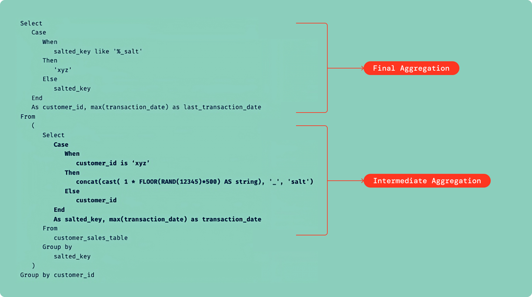
![]()
Try these solutions in the order they are mentioned above. That means salting should be the last choice, not the first, as it requires code changes. Hints and AQE solutions are much simpler to implement.

Data Explosion — Identification, Consequences and Solutions
During a Spark job execution after a certain transformation step, you may see an unusually big rise in data volume, which is considered a data explosion. The query execution is significantly slowed as a result of this. The following are some of the most prevalent transformations that can result in a data explosion:
1. Explode function
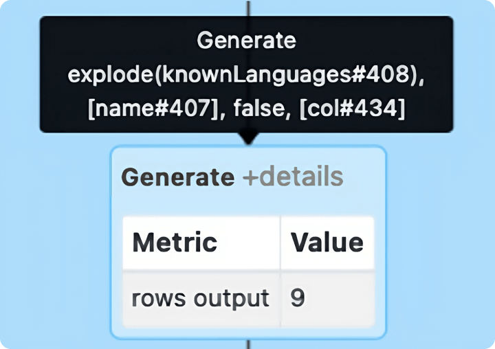
While working with structured files with the formats like JSON, Parquet, Delta and XML, we often get data in collections like arrays, lists and maps. In such cases, the explode() function is useful to convert collection columns to rows in order to process in Spark effectively. This explode operation can significantly increase the data volume. The explode operation is represented by the Generate node in Spark UI as shown in the image above.
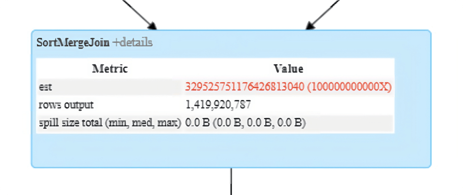
2. Join operation
A common cause of slow queries is joins that produce significantly more rows than anticipated. This is often referred to as a “row explosion.” Refer to the rows output metric in the SortMergeJoin or ShuffleHashJoin node of Spark UI to identify a potential row explosion.
Impact
While reading input data from sources like Parquet, Delta, etc., Spark approximately reads 128MB per task per core, which is a very decent partition size to fit inside the memory available to each CPU core. But due to data explosion, the 128MB data might get converted into a significantly high volume (for example, a couple of GBs), which is problematic as a single CPU core might not have enough memory to fit that exploded partition. As a consequence, for subsequent wide transformations, a lot of data might get spilled into the disk, which can significantly impact the query performance.
Solutions
- Decrease the size of input partitions, i.e.,
spark.sql.files.maxPartitionBytes(default 128MB), to create smaller input partitions in order to counter the effect ofexplode()function. Instead of 128MB, you can choose a much smaller partition size like 16MB or 32MB, for example.
- You can explicitly call the repartition() function right after the read statement to increase the total number of partitions. This will allow you to reduce the size of each partition.
- When the explosion is happening due to a join operation, a simple solution would be to increase the number of shuffle partitions, which will decrease the size of the partition to much less than 128MB. Refer to the manual shuffle partitions tuning section for more information.

Data Skipping and Pruning
The amount of data to process has a direct relationship with query performance. Therefore, it’s extremely important to read only the required data and skip all the unnecessary data. There are a couple of data skipping and pruning techniques that you can apply with Spark and Delta.
1. Delta data skipping
Delta data skipping automatically collects the stats (min, max, etc.) for the first 32 columns for each underlying Parquet file when you write data into a Delta table. Databricks takes advantage of this information (minimum and maximum values) at query time to skip unnecessary files in order to speed up the queries.
To collect stats for more than the 32 first columns, you can set the following Delta property:
Collecting statistics on long strings is an expensive operation. To avoid collecting statistics on long strings, you can either configure the table property delta.dataSkippingNumIndexedCols to avoid columns containing long strings or move columns containing long strings to a column greater than delta.dataSkippingNumIndexedCols using ALTER TABLE as shown below:
2. Column pruning
When reading a table, we generally choose all of the columns, but this is inefficient. To avoid scanning extraneous data, always inquire about what columns are truly part of the workload computation and are needed by downstream queries. Only those columns should be selected from the source database. This has the potential to have a significant impact on query performance.
3. Predicate pushdown
This aims at pushing down the filtering to the “bare metal” — i.e., a data source engine. That is to increase the performance of queries since the filtering is performed at a very low level rather than dealing with the entire data set after it has been loaded to Spark’s memory.
To leverage the predicate pushdown, all you need to do is add filters when reading data from source tables. Predicate pushdown is data source engine dependent. It works for data sources like Parquet, Delta, Cassandra, JDBC, etc., but it will not work for data sources like text, JSON, XML, etc.
In cases where you are performing join operations, apply filters before joins. As a rule of thumb, apply filter(s) right after the table read statement.
4. Partition pruning
The partition elimination technique allows optimizing performance when reading folders from the corresponding file system so that the desired files only in the specified partition can be read. It will address shifting the filtering of data as close to the source as possible to prevent keeping unnecessary data in memory with the aim of reducing disk I/O.
To leverage partition pruning, all you have to do is provide a filter on the column(s) being used as table partition(s).
In cases where you are performing join operations, apply partition filter(s) before joins. As a rule of thumb, apply partition filter(s) right after the table read statement.
5. Dynamic partition pruning (DPP)
In Apache Spark 3.0+, a new optimization called Dynamic Partition Pruning (DPP) is implemented. DPP occurs when the optimizer is unable to identify at parse time the partitions it has to eliminate. In particular, we consider a star schema that consists of one or multiple fact tables referencing any number of dimension tables. In such join operations, we can prune the partitions the join reads from a fact table by identifying those partitions that result from filtering the dimension tables. To leverage this feature, no configuration is required. It’s enabled by default on Spark 3.0+.
6. Dynamic file pruning (DFP)
Dynamic File Pruning (DFP) is available on Databricks Runtime and is by default enabled on all recent runtimes. As the name suggests, it works in a similar manner as DPP, but it performs dynamic pruning at the file level instead of the partition level to further speed up your queries. To leverage this feature, no configuration is required. DFP is automatically enabled in Databricks Runtime 6.1 and higher.

Data Caching — Leverage Caching to Speed Up the Workloads
Delta cache and Spark cache are the two different types of caching that you can leverage to make your workloads faster.
1. Delta cache
The Delta cache accelerates data reads by creating copies of remote files in nodes’ local storage (SSD drives) using a fast intermediate data format.
- Use Accelerated instances with Delta cache enabled by default (such as
Standard_E16ds_v4in the memory-optimized category andStandard_L4sin the storage-optimized category in Azure cloud) - Delta cache can be enabled on the workers of other instance families with SSD drives (such as
Fsv2-seriesin the compute-optimized category in Azure cloud). To explicitly enable the Delta caching, set the following configuration:
2. Spark cache
Using cache() and persist() methods, Spark provides an optimization mechanism to cache the intermediate computation of a Spark DataFrame so they can be reused in subsequent actions. Similarly, you can also cache a table using the CACHE TABLE command. There are different cache modes that allow you to choose where to store the cached data (in the memory, in the disk, in the memory and the disk, with or without serialization, etc.).
![]()
- Spark caching is only useful when more than one Spark action (for instance, count, saveAsTable, write, etc.) is being executed on the same DataFrame
- Databricks recommends using Delta caching instead of Spark caching, as Delta caching provides better performance outcomes. The data stored in the disk cache can be read and operated on faster than the data in the Spark cache. This is because the disk cache uses efficient decompression algorithms and outputs data in the optimal format for further processing using whole-stage code generation.
- Any compute-heavy workload (with a lot of wide transformations like joins and aggregations) would benefit from Delta caching, especially when reading from the same tables over and over. Always use Delta cache-enabled instances for those workloads.
Intermediate Results — When to Persist Them
In large pipelines spanning multiple SQL queries, we often tend to create one or many intermediate working (or temp or staging) Delta tables. This allows us to break a big query into small ones for more readability and maintainability. This strategy, however, has a negative impact on the execution duration of our job since:
- We write the staging tables to the cloud storage, which takes time
- Then we read back the staging tables from cloud storage in subsequent steps, which also takes additional time
Therefore, the better approach would be to create temp views instead of materialized Delta tables since temp views are lazily evaluated and are actually not materialized.
![]()
- Always turn an intermediate table into a temporary view if it is used only once in the same Spark job
- If an intermediate table is being used more than once in the same Spark job, you should leave it as a Delta table rather than turning it into a temporary view since using a temporary view can cause Spark to execute the related query in part more than once. It is strongly advised to use Delta cache-enabled worker instances in this situation so that the temporary table can be automatically cached in worker SSD drives to speed up the scanning.

Delta Merge — Let’s Speed It Up
You can upsert data from a source table, view or DataFrame into a target Delta table by using the MERGE operation. Delta Lake supports inserts, updates and deletes in the MERGE command.
Instead of overwriting and inserting the entire Delta table on a daily basis, it is recommended that we use an incremental load strategy wherever possible. To achieve the incremental load, Delta MERGE is very essential. Delta merge can also be used to create SCD Type 2 tables and change data capture (CDC) use cases. Here are a couple of examples of how you can use Delta merge: SCD Type 2 using Merge, Change data capture using Merge.
Merge internals
Behind-the-scenes merge operation is performed in two steps:
- Inner-join between source and target using the condition in the ON clause to return a list of files in target that contain matching rows to the driver.
- This step comprises two possibilities — depending on the conditions, one of the following will be executed:
- If there were no matching rows in the target in step 1, an append-only write is performed to append the source to target
- Else a full outer join is performed to consolidate the changes between the source being merged and the matching files produced in step 1.
Merge challenges
There are certain performance issues that can be encountered because of the following reasons:
- If we do not have a specific enough condition to match in the ON clause of the merge operation, we will end up rewriting a lot of data. This can slow down the merge.
- If we rewrite a large amount of data after each merge, the Z-order sorting will be messed up, and we may need to execute Z-order after each merge to maintain the sorting
Merge optimizations
We can use the following optimization techniques to resolve the above-mentioned challenges:
Target table data layout
If the target table contains large files (for example, 500MB-1GB), many of those files will be returned to the drive during step 1 of the merge operation, as the larger the file, the greater the chance of finding at least one matching row. And because of this, a lot of data will be rewritten. Therefore, for the merge-heavy tables, it’s recommended to have smaller file sizes from 16MB to 64MB, varying on a case-by-case basis and workload. Refer to the section on file size tuning for more details.
Partition pruning
Provide the partition filters in the ON clause of the merge operation to discard the irrelevant partitions. Refer to this example for more details.
File pruning
Provide Z-order columns (if any) as filters in the ON clause of the merge operation to discard the irrelevant files. You can add multiple conditions using the AND operator in the ON clause.
Broadcast join
Since Delta merge performs joins behind the scene, you can speed it up by explicitly broadcasting the source DataFrame to be merged in the target Delta table if the source DataFrame is small enough (<= 200MB). Refer to the broadcast join section for more information.
Low shuffle merge
- This is a new MERGE algorithm that aims to maintain the existing data organization (including Z-order clustering) for unmodified data, while simultaneously improving performance
- With this “low shuffle” MERGE, only updated rows will be reorganized by the operation, while unchanged rows remain in the same order and file grouping they were in before the operation
Low shuffle merge is enabled by default in Databricks Runtime 10.4 and above. In earlier supported Databricks Runtime versions, it can be enabled by setting the configuration spark.databricks.delta.merge.enableLowShuffle to true.
Data Purging — What to Do With Stale Data
Delta comes with a VACUUM feature to purge unused older data files. It removes all files from the table directory that are not managed by Delta, as well as data files that are no longer in the latest state of the transaction log for the table and are older than a retention threshold. The default threshold is 7 days.
You can change the default retention threshold if needed as follows:
VACUUM will skip all directories that begin with an underscore (_), which includes the _delta_log. Log files are deleted automatically and asynchronously after checkpoint operations. The default retention period of log files is 30 days, configurable through the delta.logRetentionDuration.
![]()
- It is recommended that you set a retention interval to be at least 7 days because old snapshots and uncommitted files can still be in use by concurrent readers or writers to the table. If VACUUM cleans up active files, concurrent readers can fail, or, worse, tables can be corrupted when VACUUM deletes files that have not yet been committed.
- Set
deltaTable.deletedFileRetentionDurationanddelta.logRetentionDurationto the same value to have the same retention for data and transaction history - Run the VACUUM command on a daily/weekly basis depending on the frequency of transactions applied on the Delta tables
- Never run this command as part of your job but run it as a separate job on a dedicated job cluster, usually clubbed with the OPTIMIZE command
- VACUUM is not a very intensive operation (the main task is file listing, which is done in parallel on the workers; the actual file deletion is handled by the driver), so a small autoscaling cluster of 1 to 4 workers is sufficient
Delta Live Tables (DLT)
Delta Live Tables (DLT) makes it easy to build and manage reliable batch and streaming data pipelines that deliver high-quality data on the Databricks Lakehouse Platform.
DLT helps data engineering teams simplify ETL development and management with declarative pipeline development, automatic data testing, and deep visibility for monitoring and recovery.
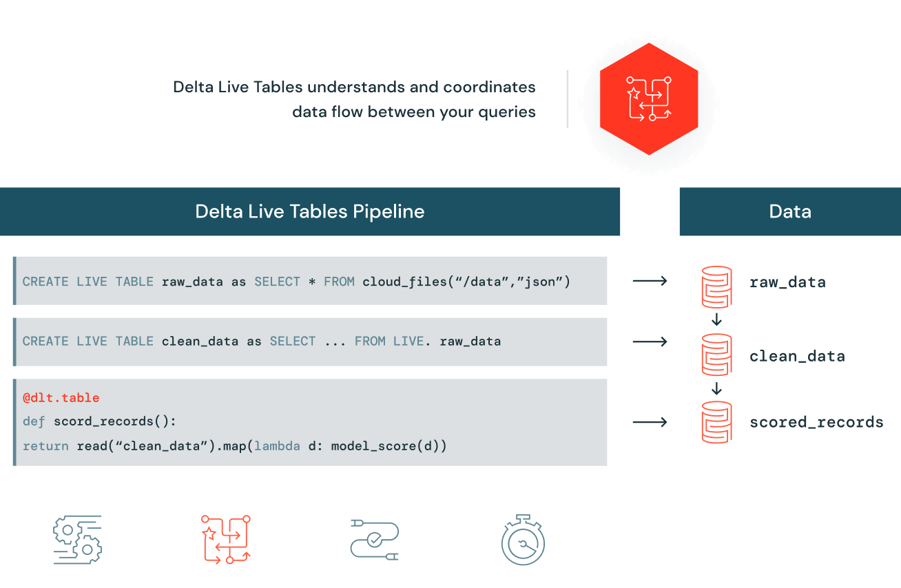
Easily build and maintain data pipelines
With Delta Live Tables, easily define end-to-end data pipelines in SQL or Python. Simply specify the data source, the transformation logic and the destination state of the data — instead of manually stitching together siloed data processing jobs. Automatically maintain all data dependencies across the pipeline and reuse ETL pipelines with environment-independent data management. Run in batch or streaming mode and specify incremental or complete computation for each table.
Automatic data quality testing
Delta Live Tables helps to ensure accurate and useful BI, data science and machine learning with high-quality data for downstream users. Prevent bad data from flowing into tables through validation and integrity checks and avoid data quality errors with predefined error policies (fail, drop, alert or quarantine data). In addition, you can monitor data quality trends over time to get insight into how your data is evolving and where changes may be necessary.
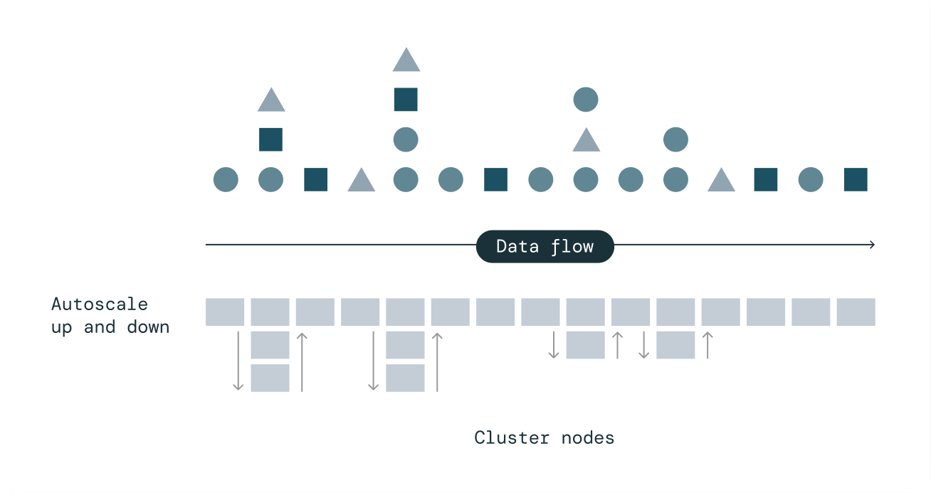
Cost-effective streaming through efficient compute autoscaling
Delta Live Tables Enhanced Autoscaling is designed to handle streaming workloads that are spiky and unpredictable. It optimizes cluster utilization by only scaling up to the necessary number of nodes while maintaining end-to-end SLAs and gracefully shuts down nodes when utilization is low to avoid unnecessary spending.
Deep visibility for pipeline monitoring and observability
Gain deep visibility into pipeline operations with tools to visually track operational stats and data lineage. Reduce downtime with automatic error handling and easy replay. Speed up maintenance with single-click deployment and upgrades.
![]()
- DLT is a managed ETL framework that frees users to concentrate on writing business-related code while DLT handles operational tasks including clusters, autoscaling, retries on failures, and other configuration tweaking in the background. Therefore, it is advised to use DLT for data engineering workloads as much as possible so that users are spared from worrying about Spark tuning, cluster configuration and tuning (see the following part), Delta maintenance tasks, etc.
Databricks Cluster Configuration and Tuning
All-purpose clusters vs. automated clusters
- All-purpose clusters should only be used for ad hoc query execution and interactive notebook execution during the development and/or testing phases
- Never use an all-purpose cluster for an automated job; instead, use ephemeral (also called automated) job clusters for jobs
- This is the single biggest cost optimization impact: you could reduce the DBU cost by opting for an automated cluster instead of an all-purpose cluster
- You can also leverage SQL warehouses to run your SQL queries. A SQL warehouse is a compute resource that lets you run SQL commands on data objects within Databricks Lakehouse. SQL warehouses are also available in serverless flavor, offering you access to an instant compute.
Autoscaling
Databricks provides a unique feature of cluster autoscaling. Here are some guidelines on when and how to leverage autoscaling:
- Always use autoscaling when running ad hoc queries, interactive notebook execution, and developing/testing pipelines using interactive clusters with minimum workers set to 1. The combination of both can bring good cost savings.
- For an autoscaling job cluster in production, don't set the minimum instances to 1 if the job certainly needs more resources than 1 worker. Instead, set it to a bigger value based on the minimum compute requirements. It will save you some scale-up time.
- You don't necessarily need to employ autoscaling if you've fine-tuned the Spark shuffle partitions to use all of the worker cores for a given job and that job has its own job cluster. This is the best option because it allows complete cost control. However, you can still use autoscaling if you wish to have a computational resource buffer in case of unexpected data surges. For this choose the minimum number of workers based on the projected daily data load and required SLA and simply keep a couple of additional workers (say, 2 to 4) as a buffer to be added by autoscaling if and when needed.
- Workflows in Databricks allow you to share a job cluster with many tasks (jobs) that are all part of the same pipeline. If many jobs are executing in parallel on a shared job cluster, autoscaling for that job cluster should be enabled to allow it to scale up and supply resources to all of the parallel jobs.
- Autoscaling should not be used for Spark Structured Streaming workloads because once the cluster scales up, it is tough to determine when to scale it down. There were some advances made in this aspect in Delta Live Tables, and autoscaling works pretty well for steaming workloads in Delta Live Tables thanks to the feature called Enhanced Autoscaling.
Instance types based on workloads
General guidelines to choose instance family based on the workload type:
| VM Category | Workload Type |
|---|---|
| Memory Optimized |
|
| Compute Optimized |
|
| Storage Optimized |
|
| GPU Optimized |
|
| General Purpose |
|
Number of workers
Choosing the right number of workers requires some trials and iterations to figure out the compute and memory needs of a Spark job. Here are some guidelines to help you start:
- Never choose a single worker for a production job, as it will be the single point for failure
- Start with 2-4 workers for small workloads (for example, a job with no wide transformations like joins and aggregations)
- Start with 8-10 workers for medium to big workloads that involve wide transformations like joins and aggregations, then scale up if necessary
- Fine-tune the shuffle partitions when applicable to fully engage all cluster cores
- The approximate execution time can be determined after a few first executions. If this violates the SLA, you should add more workers.
- Remember that if shuffle partitions are fine-tuned and data skew and spill issues are addressed, adding additional workers will not result in a higher cost. In this situation, adding more workers will proportionally reduce the total execution time, resulting in a cost that is more or less the same.
Spot instances
- Use spot instances to use spare VM instances for a below-market rate
- Great for interactive ad hoc/shared clusters
- Can use them for production jobs without SLAs
- Not recommended for production jobs with tight SLAs
- Never use spot instances for the driver
Auto-termination
- Terminates a cluster after a specified inactivity period in minutes for cost savings
- Enable auto-termination for all-purpose clusters to prevent idle clusters from running overnight or on weekends
- Clusters are configured to auto-terminate in 120 minutes by default, but you can change this to a much lower value, such as 10-15 minutes, to further save cost
Cluster usage
We need to make sure we're getting the most out of our cluster. A job may run many iterations on a cluster to complete depending on the number of shuffle partitions, so the rule of thumb is to ensure that all worker cores are actively occupied and not idle in any of the iterations. The only way to be absolutely certain is to always set the number of shuffle partitions as a multiplication of the total number of worker cores.
Ganglia UI is your friend to make sure that all the cores are fully engaged. Ganglia UI can be accessed right from the cluster UI pinned under the metrics tab.
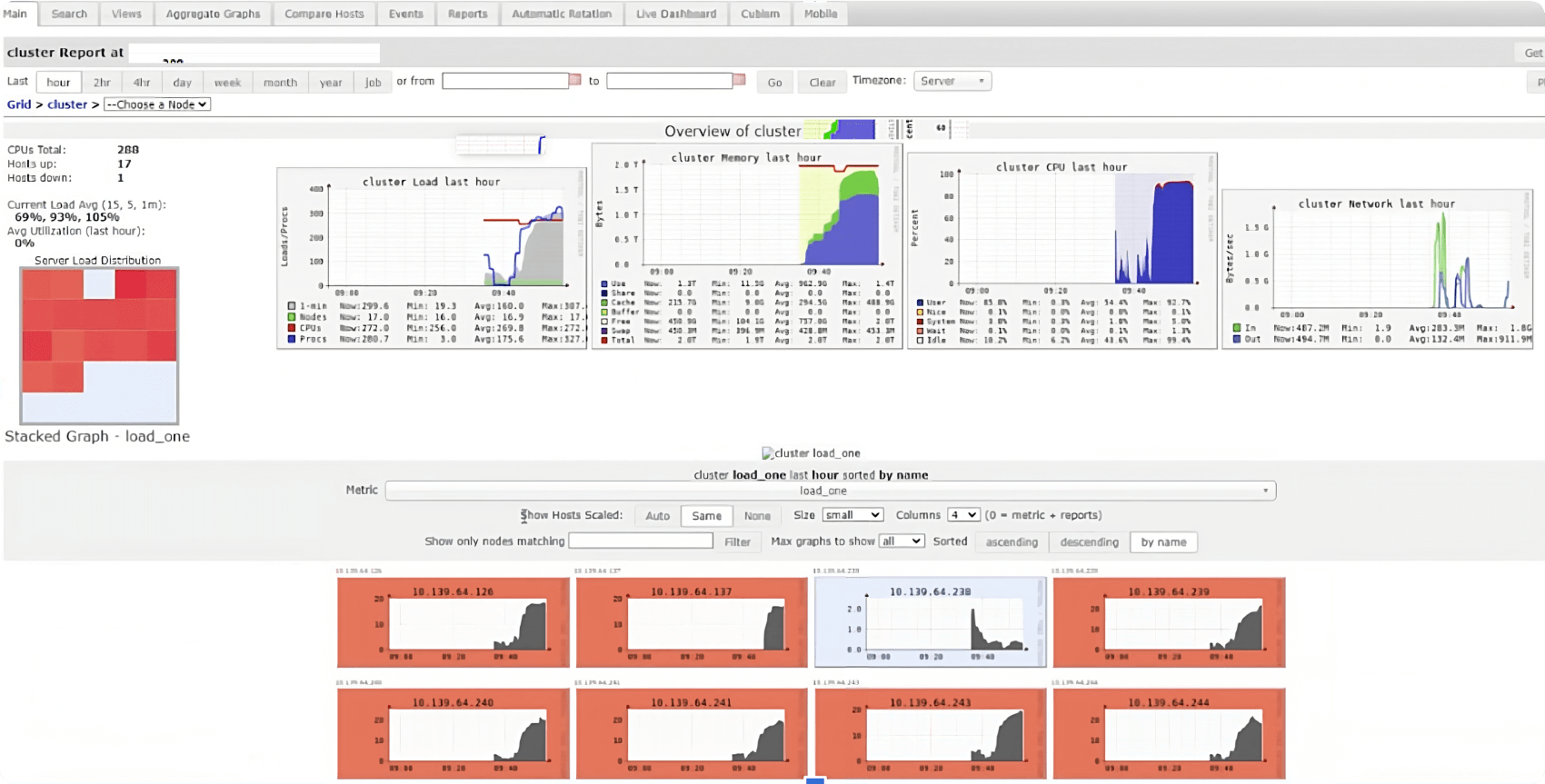
Things to pay attention to in the Ganglia UI:
- The average cluster load should always be greater than 80%
- During query execution, all squares in the cluster load distribution graph (on the left in the UI) should be red (with the exception of the driver node), indicating that all worker cores are fully engaged
- The use of cluster memory should be maximized (at least 60%-70%, or even more)
- Ganglia metrics are only available for Databricks Runtime 12.2 and below
Ganglia has been replaced in Databricks Runtime 13 and above by a new cluster metrics UI that is more secure and powerful, and provides a simple user experience with a clean design. Therefore, in DBR 13 and above, you can leverage this new UI to check out the cluster utilization.
Cluster policy
A cluster policy limits the ability to configure clusters based on a set of rules. Effective use of cluster policies allows administrators to:
- Limit users to create clusters with prescribed settings
- Control cost by limiting per-cluster maximum cost (by setting limits on attributes whose values contribute to hourly price)
- Simplify the user interface and enable more users to create their own clusters (by fixing and hiding some values)
Refer to the cluster policies best practice guide to plan and ensure a successful cluster governance rollout.
Instance pools
Databricks pools reduce cluster start and autoscaling times by maintaining a set of idle, ready-to-use instances. When a cluster is attached to a pool, cluster nodes are created using the pool’s idle instances. When instances are idle in the pool, they only incur Azure VM costs and no DBU costs.
Pools are recommended for workloads with tight SLAs, where fast access to additional compute resources is a requirement (i.e., fast autoscaling) to improve processing time while minimizing cost.
Photon
Photon is the next-generation engine on the Databricks Lakehouse Platform that provides extremely fast query performance at a low cost. Photon is compatible with Apache Spark APIs, works out of the box with existing Spark code, and provides significant performance benefits over the standard Databricks Runtime. Following are some of the advantages of Photon:
- Accelerated queries that process a significant amount of data (> 100GB) and include aggregations and joins
- Faster performance when data is accessed repeatedly from the Delta cache
- More robust scan/read performance on tables with many columns and many small files
- Faster Delta writing using UPDATE, DELETE, MERGE INTO, INSERT, and CREATE TABLE AS SELECT
- Join improvements
It is recommended to enable Photon (after evaluation and performance testing) for workloads with the following characteristics:
- ETL pipelines consisting of Delta MERGE operations
- Writing large volumes of data to cloud storage (Delta/Parquet)
- Scans of large data sets, joins, aggregations and decimal computations
- Auto Loader to incrementally and efficiently process new data arriving in storage
- Interactive/ad hoc queries using SQL
Others
- Use the latest LTS version of Databricks Runtime (DBR), as the latest Databricks Runtime is almost always faster than the one before it
- Restart all-purpose clusters periodically, at least once per week (or even daily on busy clusters), as some older DBRs might have stuck/zombie Spark jobs
- Configure a large driver node (4-8 cores and 16-32GB is mostly enough) only if:
- Large data sets are being returned/collected (
spark.driver.maxResultSizeis typically increased also) - Large broadcast joins are being performed
- Many (50+) streams or concurrent jobs/notebooks on the same cluster:
- Delta Live Tables might be a better fit for such workloads, as DLT determines the complete DAG of the pipeline and then goes about running it in the most optimized way possible
- Large data sets are being returned/collected (
- For workloads using single-node libraries (e.g., Pandas), it is recommended to use single-node data science clusters as such libraries do not utilize the resources of a cluster in a distributed manner
- Cluster tags can be associated with Databricks clusters to attribute costs to specific teams/departments as they are automatically propagated to underlying cloud resources (VMs, storage and network, etc.)
- For such shuffle-heavy workloads, it is recommended to use fewer larger node sizes, which will help with reducing network I/O when transferring data between nodes
- Choosing workers with a large amount of RAM (>128GB) can help jobs perform more efficiently but can also lead to long pauses during garbage collection, which negatively impacts the performance and in some cases can cause job failure. Therefore, it’s not recommended to choose workers with more than 128GB RAM. Apart from worker memory, there are some other ways to avoid long garbage collection (GC) pauses:
- Don’t call
collect()functions to collect data on the driver- Applies to the toPandas() function as well
- Prefer Delta cache over Spark cache
- If none of the above solutions help, use G1GC garbage collector instead by setting
spark.executor.defaultJavaOptionsandspark.executor.extraJavaOptionsto-XX:+UseG1GCvalue in Spark config section under Advance cluster options
- Don’t call
- Please refer to the Cluster sizing examples in Databricks documentation for specific cluster sizing examples
Conclusion
We have covered many Spark, Delta and Databricks optimization strategies and tactics in this book. The purpose of this book is to make readers aware of different challenges that they could encounter when developing big data workloads to run on distributed compute, as well as the methods for identifying these difficulties and solutions for them. A guide like this may truly assist data engineers and data architects in taking control of the cost of engineering and SLAs and making the best use of cloud resources in the present economic climate, where every enterprise is attempting to cut costs and do more with less.
Databricks is the data and AI company. More than 9,000 organizations worldwide — including Comcast, Condé Nast and over 50% of the Fortune 500 — rely on the Databricks Lakehouse Platform to unify their data, analytics and AI. Databricks is headquartered in San Francisco, with offices around the globe. Founded by the original creators of Apache Spark™, Delta Lake and MLflow, Databricks is on a mission to help data teams solve the world’s toughest problems. To learn more, follow Databricks on Twitter, LinkedIn and Facebook.
© Databricks 2023. All rights reserved. Apache, Apache Spark, Spark and the Spark logo are trademarks of the Apache Software Foundation. Privacy Policy | Terms of Use