How to Manage End-to-end Deep Learning Pipelines with Databricks

Deep Learning (DL) models are being applied to use cases across all industries -- fraud detection in financial services, personalization in media, image recognition in healthcare and more. With this growing breadth of applications, using DL technology today has become much easier than just a few short years ago. Popular DL frameworks such as Tensorflow and Pytorch have matured to the point where they perform well and with a great deal of precision.  Machine Learning (ML) environments like Databricks' Lakehouse Platform with managed MLflow have made it very easy to run DL in a distributed fashion, using tools like Horovod and Pandas UDFs.  

Challenges

One of the key challenges remaining today is how to best automate and operationalize DL machine learning pipelines in a controlled and repeatable fashion. Technologies such as Kubeflow provide a solution, but they are often heavyweight, require a good amount of specific knowledge, and there are few managed services available -- which means that engineers have to manage these complex environments on their own. It would be much simpler to have the management of the DL pipeline integrated into the data and analytics platform itself.

This blog post will outline how to easily manage DL pipelines within the Databricks environment by utilizing Databricks Jobs Orchestration, which is currently a public preview feature. Jobs Orchestration makes managing multi-step ML pipelines, including deep learning pipelines, easy to build, test and run on a set schedule. Please note that all code is available in this GitHub repo. For instructions on how to access it, please see the final section of this blog.

Let’s look at a real-world business use case. CoolFundCo is a (fictional) investment company that analyses tens of thousands of images every day in order to identify what they represent and categorize the content. CoolFundCo uses this technique in a variety of ways: for example, to look at pictures from malls around the country to determine short-term economic trends. The company then uses this as one of the data points for investments. The data scientists and ML engineers at CoolFundCo spend a lot of time and effort managing this process. CoolFundCo has a large stock of existing images, and every day they get a large batch of new images sent to their cloud object storage (in this example Microsoft Azure Data Lake Storage (ADLS)), but it could also be AWS S3 or Google Cloud Storage (GCS).

Currently, managing that process is a nightmare. Every day, their engineers copy the images, run their deep learning model to predict the image categories, and then share the results by saving the output of the model in a CSV file. The DL models have to be verified and re-trained on a regular basis to ensure that the quality of the image recognition is maintained, which is also currently a manual process conducted by the team in their own development environments. They often lose track of the latest and best versions of the underlying ML models and which images they used to train the current production model. The execution of the pipelines happens in an external tool, and they have to manage different environments to control the end-to-end flow.

Solution

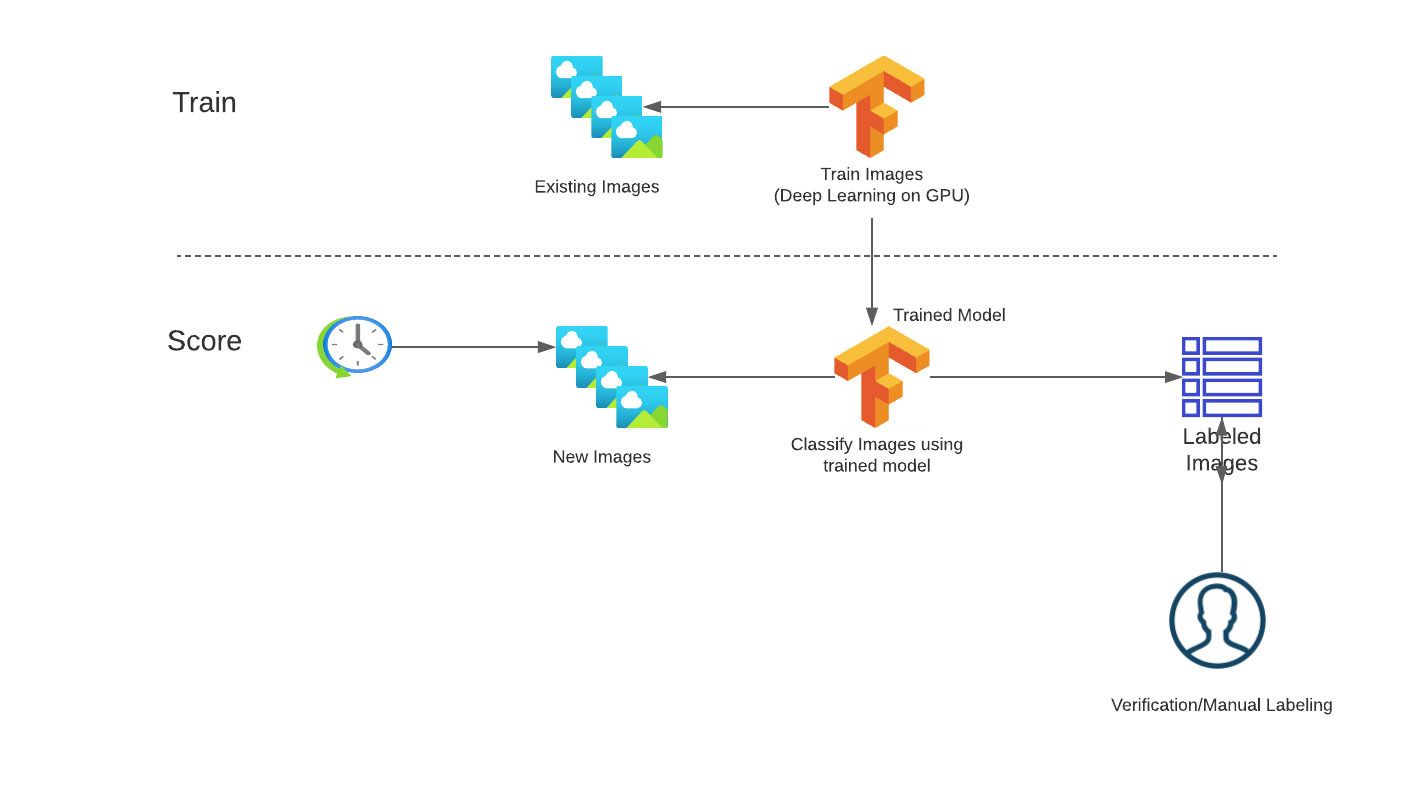
In order to bring order to the chaos, CoolFundCo is adopting Databricks to automate the process. As a start, they separate the process into a training and scoring workflow.

In the training workflow, they need to:

1. Ingest labeled images from cloud storage into the centralized lakehouse
2. Use existing labeled images to train the machine learning model
3. Register the newly trained model in a centralized repository

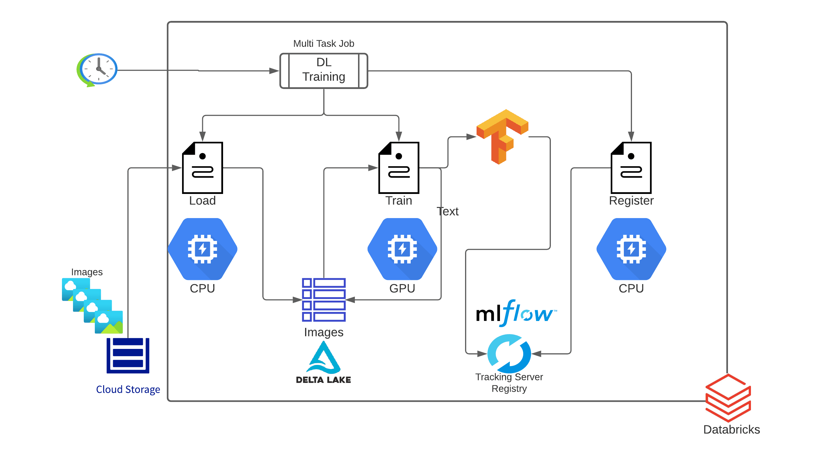
Each of their workflows consists of a set of tasks to achieve the desired outcome. Each task uses different sets of tools and functionality and therefore requires different resource configurations (cluster size, instance type, CPU vs. GPU, etc.). They decide to implement each of these tasks in a separate Databricks notebook. The resolution architecture is depicted in Figure 2:

The scoring workflow is made up of the following steps:

1. Ingest new images from cloud storage into the centralized lakehouse
2. Score each image using the latest model from the repository as fast as possible
3. Store the scoring results in the centralized lakehouse
4. Send a subset of the images to a manual labeling service to verify the accuracy

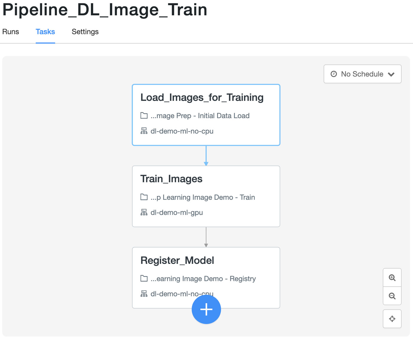
DL training pipeline

Let’s take a look at each task of the training pipeline individually :

1. Ingest labeled images from cloud storage into the centralized data lake  [Desired Infrastructure: Large CPU Cluster]

The first step in the process is to load the image data into a usable format for the model training. They load all of the training data (i.e., the new images) using Databricks Auto Loader, which  incrementally and efficiently processes new data files as they arrive in cloud storage.  The Auto Loader feature helps data management and automatically handles continuously arriving new images. CoolFundCo's team decides to use Auto Loader’s 'trigger once' functionality, which allows the Auto Loader streaming job to start,  detect any new image files since the last training job ran, load only those new files and then turn off the stream.  They load all of the images using Apache Spark’s™  binaryFile reader and parse the label from the file name and store that as its own column. The binaryFile reader converts each image file into a single record in a DataFrame that contains the raw content, as well as metadata of the file. The DataFrame will have the following columns:

• path (StringType): The path of the file.
• modificationTime (TimestampType): The modification time of the file. In some Hadoop FileSystem implementations, this parameter might be unavailable, and the value would be set to a default value.
• length (LongType): The length of the file in bytes.
• content (BinaryType): The contents of the file.

They then write all of the data into a Delta Lake table, which they can access and update throughout the rest of their training and scoring pipelines. Delta Lake adds reliability, scalability, security and performance to data lakes and allows for data warehouse- like access using standard SQL queries -- which is why this type of architecture is also referred to as a lakehouse. Delta Tables automatically add version control, so each time the table is updated, a new version will indicate which images have been added.

2. Use existing labeled images to train the machine learning model  [Desired Infrastructure: GPU Cluster]

The second step in the process is to use their pre-labeled data to train the model. They can use Petastorm,  an open source data access library that allows for the training of deep learning models directly from Parquet files and Spark DataFrames. They read the  Delta table of images directly into a Spark Dataframe, process each image to the correct shape and format and then use Petastorm’s Spark Converter to generate the input features for their model.

In order to scale deep learning training, they want to take advantage of not just a single large GPU, but a cluster of GPUs. On Databricks, this can be done simply by importing and using HorovodRunner, a general API to run distributed deep learning workloads on a Spark Cluster using Uber’s Horovod framework.

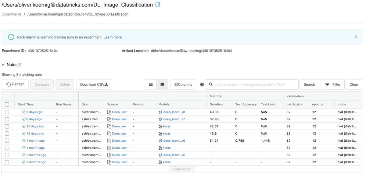
Using MLflow, the team is able to track the entire model training process, including hyperparameters, training duration, loss and accuracy metrics, and the model artifact itself, to an MLflow experiment. The MLflow API has auto-logging functionality for the most common ML libraries, including Spark MLlib, Keras, Tensorflow, SKlearn and XGBoost. This feature automatically logs model-specific metrics, parameters and model artifacts. On Databricks, when using a Delta training data source, auto-logging also tracks the version of data being used to train the model, which allows for easy reproducibility of any training run on the original dataset.

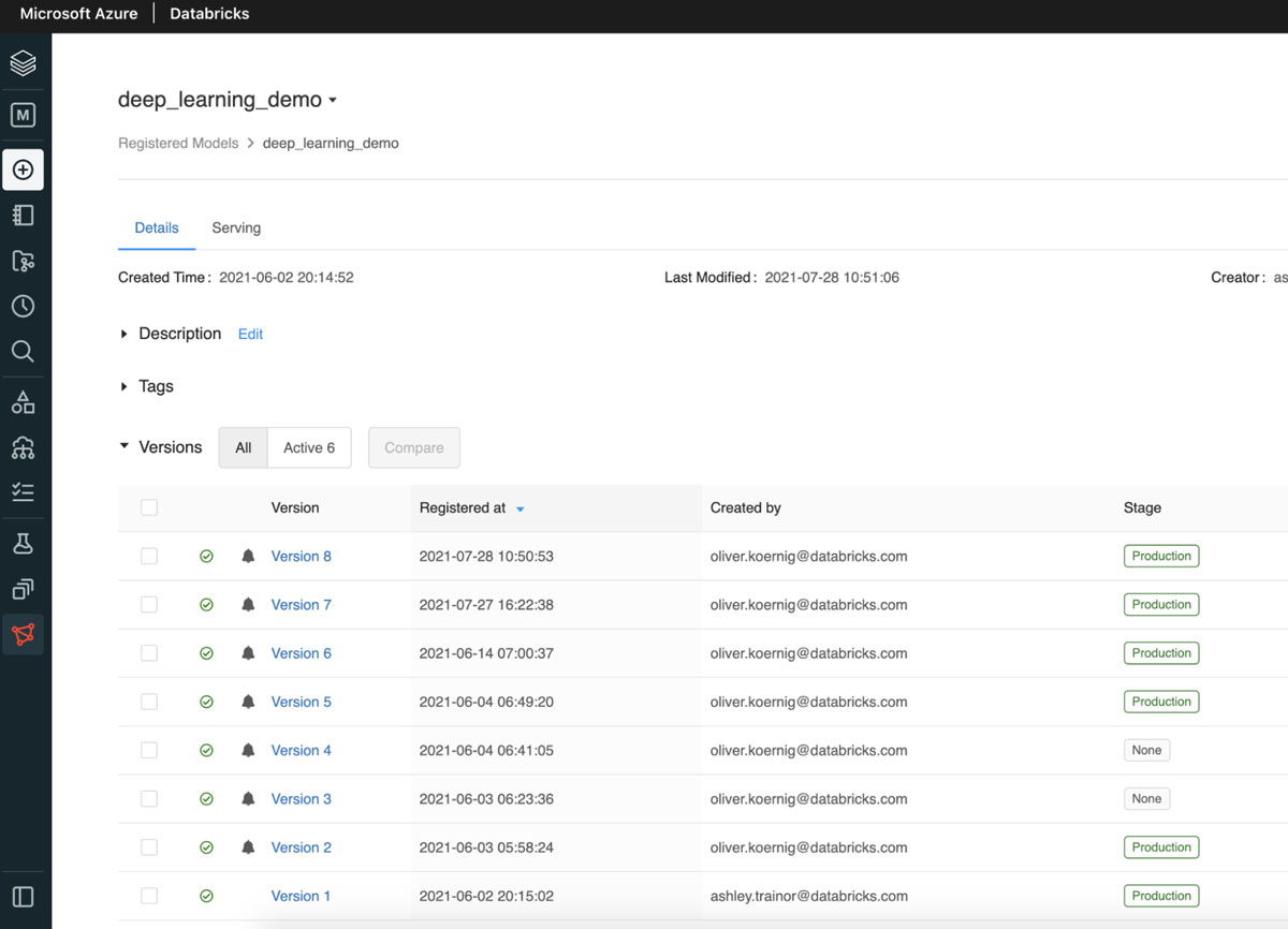
3. Register the newly trained model in the MLflow Registry - [Desired Infrastructure: Single Node CPU Cluster]

The final step in their model training pipeline is to register the newly trained model in the Databricks Model Registry. Using the artifact stored in the previous training step, they can create a new version of their image classifier. As the model is transitioned from a new model version to staging and then production, they can develop and run other tasks that can validate model performance, scalability and more.  The Databricks Models UI shows the latest status of the model (see below).

Scoring pipeline

Next, we can look at the steps in CoolFundCo’s scoring pipeline:

1. Ingest new unlabeled images from cloud storage into the centralized data lake [Desired Infrastructure: Large CPU Cluster]

The first step in the scoring process is to load the newly landed image data into a usable format for the model to classify. They load all of the new images using Databricks Auto Loader. CoolFundCo's team again decides to use Auto Loader’s trigger once functionality, which allows the Auto Loader streaming job to start, detect any new image files since the last scoring job ran,  load only those new files and then  turn off the stream. In the future, they can opt to change this job to run as a continuous stream. In that case, new images that are landed in their cloud storage will be picked up and sent to the model for scoring as soon as they arrive.

As the last step, all the unlabeled images are stored in a Delta Lake table, which can be accessed and updated throughout the rest of their scoring pipeline.

2. Score new images and update their predicted labels in the Delta table [Desired Infrastructure: GPU Cluster]

Once the new images are loaded into our Delta table, they can run our model scoring notebook. This notebook takes all of the records (images) in the table that do not have a label or predicted label yet, loads the production version of the classifier model that was trained in our training pipeline, uses the model to classify each image and then updates the Delta table with the predicted labels. Because we are using the Delta format, we can use the MERGE INTO command to update all records in the table that have new predictions.

3. Send images to be manually labeled by Azure [Desired Infrastructure: Single Node CPU]

CoolFundCo uses the Azure Machine Learning labeling service  to manually label a subset of new images. Specifically, they sample the images for which the DL model can't make a very confident decision -- less than 95% certain about the label. They can then select those images easily from the Delta table, where all of the images, image metadata and label predictions are being stored as a result of the scoring pipeline. Those images are then written to a location being used as the labeling service’s datastore. With the labeling service’s incremental refresh, the images to be labeled are found by the labeling project and labeled. The output of the labeling service can then be reprocessed by Databricks and MERGED into the Delta table, populating the label field for the image.

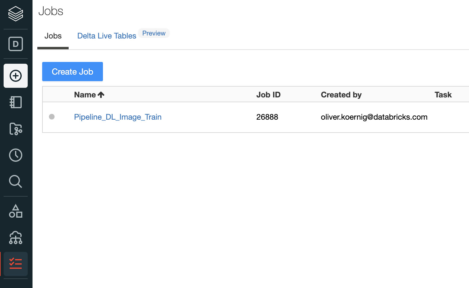
Workflow deployment

Once the training, scoring, and labeling task notebooks have been tested successfully, they can be put into the production pipelines. These pipelines will run the training, scoring and labeling processes in regular intervals (e.g., daily, weekly, bi-weekly or monthly) based on the team’s desired schedule. For this functionality, Databricks' new Jobs Orchestration feature is the ideal solution, as it enables you to reliably schedule and trigger sequences of Jobs that contain multiple tasks with dependencies. Each notebook is a task, and their overall training pipeline, therefore, creates a Directed Acyclic Graph (DAG). This is a similar concept to what open source tools like Apache Airflow create; however, the benefit is that the entire end-to-end process is completely embedded within the Databricks environment, and thus makes it very easy to manage, execute and monitor these processes in one place.

Setting up a task

Each step or “task” in the workflow has its own assigned Databricks Notebook and cluster configuration. This allows each step in the workflow to be executed on a different cluster with a different number of instances, instance types (memory vs compute optimized, CPU vs. GPU), pre-installed libraries, auto-scaling setting and so forth. It also allows for parameters to be configured and passed to individual tasks.

In order to use the Jobs Orchestration public preview feature, it has to be enabled in the Databricks Workspace by a workspace  admin.  It will replace the existing (single task) jobs feature and cannot be reversed. Therefore it’s best to try this in a separate Databricks workspace if possible as there could potentially be compatibility issues with previously defined single tasks jobs.

The image scoring workflow is a separate Jobs Orchestration pipeline that will be executed once a day. As GPUs may not provide enough of an advantage for image scoring, all the nodes use regular CPU-based Compute clusters.

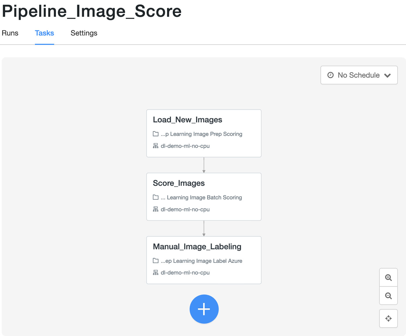
Lastly, in order to further improve and validate the accuracy of the classification, the scoring workflow picks a subset of the images and makes them available to a manual image labeling service. In this example, we are using Azure ML's manual labeling services. Other cloud providers offer similar services.

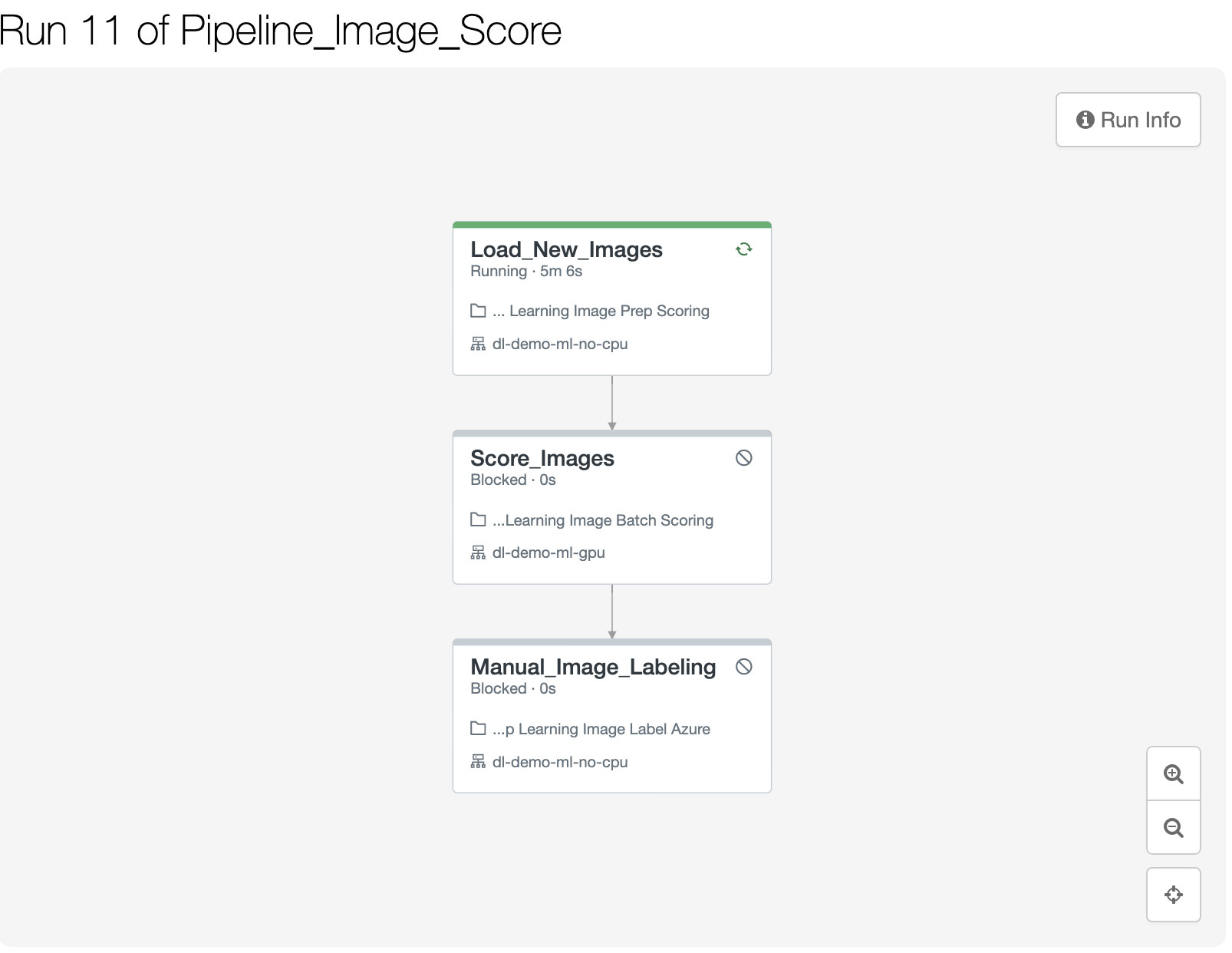
Executing and monitoring the Jobs Orchestration pipelines

When Jobs Orchestration pipelines are executed, users can  view progress in real time in the Jobs viewer.  This allows for an easy check if the pipelines are running correctly and how much time has passed.

For more info on how to manage Jobs Orchestration pipelines, please refer to the online documentation.

Conclusion

After implementing the DL pipelines in Databricks, CoolFundCo was able to solve their key challenges:

• All images and their labels are stored in a centralized and managed location and are easy to access for engineers, data scientists and analysts alike.
• New and improved versions of the model are managed and accessible in a central repository (MLflow registry).  There is no more confusion about which models are properly tested or are the most current and which ones can be used in production.
• Different pipelines (training and scoring) can run at different times while using different compute resources, even within the same workflow.
• By using Databricks Jobs Orchestration, the execution of the pipelines happens in the same Databricks environment and is easy to schedule, monitor and manage.

Using this new and improved process, the data scientists and ML engineers can now focus on what’s truly important – gaining deep insights to – rather than waste time wrangling ML Ops-related issues.

Getting started

All the code from this blog can be found in the following GitHub repository

​​https://GitHub.com/koernigo/databricks_dl_demo

Simply clone the repo into your workspace by using the Databricks Repos feature.

---

Notes

The images used in the demo are based on the Caltech256 dataset, which can be accessed using Kaggle e.g. the dataset is stored in the Databricks File System (DBFS) under /tmp/256_ObjectCategories/.  An example of how to download and install the dataset using a Databricks Notebook is provided in the repo:
https://github.com/koernigo/databricks_dl_demo/blob/main/Create%20Sample%20Images.py

There is a setup notebook that is also provided in the repo.  It contains the DDL for the Delta table used throughout the pipelines. It also separates a subset of our image data downloaded from Kaggle in the step above into a separate scoring folder. This folder is at the DBFS location /tmp/unlabeled_images/256_ObjectCategories/ and will represent a location where unlabeled images land when they need to be scored by the model

This notebook can be found in the repo here:
https://github.com/koernigo/databricks_dl_demo/blob/main/setup.py

The training and scoring jobs are also included in the repo, represented as JSON files.

The Jobs Orchestration UI currently does not allow the creation of the job via JSON using the UI. If you would like to use the JSON from the repo, you will need to install the Databricks CLI.

Once the CLI is  installed and configured, please follow these steps to replicate the jobs in your Databricks workspace:

 

1. Clone repo locally (command line):
   git clone https://github.com/koernigo/databricks_dl_demo
   cd databricks_dl_demo
2. Create GPU and non-gpu (CPU clusters:
   For this demo, we use a GPUenabled cluster and a CPUbased one.  Please create two clusters. Example cluster specs can be found here:
   https://github.com/koernigo/databricks_dl_demo/blob/main/dl_demo_cpu.json
   https://github.com/koernigo/databricks_dl_demo/blob/main/dl_demo_ml_gpu.json
   Please note that certain features in this cluster spec are Azure Databricks specific (e.g., node types). If you are running the code on AWS or GCP, you will need to use equivalent GPU/CPU node types.
3. Edit the  JSON job spec
   Select the job JSON spec you want to create, e.g., the training pipeline (https://github.com/koernigo/databricks_dl_demo/blob/main/Pipeline_DL_Image_train.json). You need to replace the cluster-ids of all the clusters with the clusters you created in the previous step (CPU and  GPU)
4. Edit the Notebook path
   In the existing JSON the repo path is /Repos/[email protected]/… Please find and replace them with the repos path in your workspace  (usually /Repos/

    

5. Create the job using the Databricks CLI
   databricks jobs create --json-file Pipeline_DL_Image_train.json --profile
6. Verify in the Jobs UI that your job was created successfully