Best Practices for Cost Management on Databricks

This blog is part of our Admin Essentials series, where we'll focus on topics important to those managing and maintaining Databricks environments. Keep an eye out for additional blogs on additional topics, and see our previous blogs on Workspace and Admin best practices!

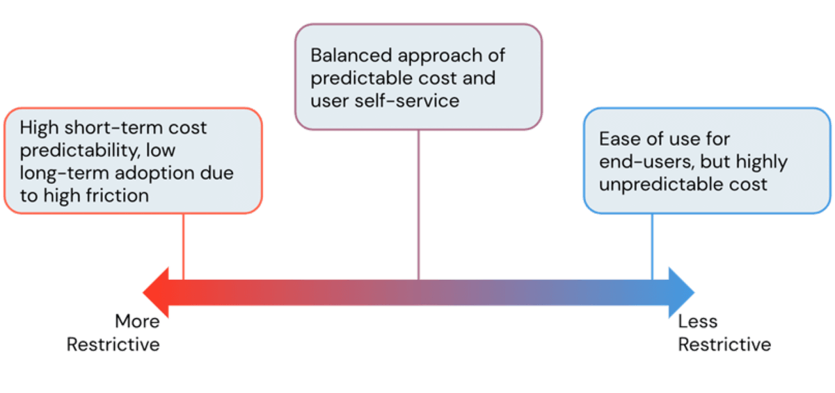
One of the main advantages of using a cloud platform is its flexibility. The Databricks Lakehouse Platform provides users easy access to near instant and horizontally scalable compute. However, with this ease of creating compute resources comes a risk of spiraling cloud costs when it's left unmanaged and without guardrails. As admins, we're always looking to strike the perfect balance of avoiding exorbitant infrastructure costs while at the same time allowing users to work without unnecessary friction. In this blog, we'll discuss Databricks Admin tools to find this balance and control costs without throttling user productivity.

What is a DBU?

Before jumping into cost controls available on the Databricks platform, it's important to first understand the cost basis of running a workload. A Databricks Unit (DBU) is the underlying unit of consumption within the platform. With the exception of a SQL Warehouse, the amount of DBUs consumed is based on the number of nodes and the computational power of the underlying VM instance types that are part of the respective cluster (as SQL warehouses are essentially a group of clusters, the DBU rate is the sum DBU rates of the clusters making up the endpoint). At the highest level, each cloud will have slightly different DBU rates for similar clusters (since node types vary across clouds), but the Databricks website has DBU calculators for each supported cloud provider (AWS | Azure | GCP).

To convert DBU usage to dollar amounts, you'll need the DBU rate of the cluster, as well as the workload type that generated the respective DBU (ex. Automated Job, All-Purpose Compute, Delta Live Tables, SQL Compute, Serverless Compute) and the subscription plan tier (Standard and Premium for Azure and GCP; Standard, Premium, and Enterprise for AWS). For example, an Enterprise Databricks workspace has a Jobs DBU list rate at 20 cents/DBU on AWS. With an instance type which runs at 3 DBU/hour, a 4 node jobs cluster would be charged at $2.40 ($0.2 * 3 * 4) for an hour. DBU calculators can be used to calculate total charges and list prices are summarized in a cloud-specific matrix including SKU and tier (AWS | Azure | GCP).

Since costs are calculated through the usage of compute resources, and more specifically clusters, it's vital to manage Databricks workspaces through cluster policies. The next section will discuss how different attributes of cluster policies can restrict DBU consumption and effectively manage costs of the platform. The proceeding sections will also review some of the underlying cloud costs to consider as well as how to monitor Databricks usage and billing.

Managing costs through cluster policies

What are cluster policies?

A cluster policy allows an admin to control the set of configurations that are available when creating a new cluster and these policies can be assigned to individual users or user groups. By default, all users have the "allow unrestricted cluster creation" entitlement within a workspace. This permission should seldom be used as it enables the user to create clusters without any restrictions outside of the assigned policies potentially leading to unmanaged and runaway costs.

Within a policy, an admin can restrict each configuration setting through an unchangeable fixed value, a more permissive range of values and regex, or a completely open default value. Policies effectively limit the amount of DBUs that can be consumed by a single cluster through restrictions on everything from more granular settings such as VM instance types to more high level "synthetic" attributes such as the max allowed DBUs per hour or cluster workload types.

Though at an initial glance it may seem that more restrictive clusters lead to lower costs, this is not always the case. Very restrictive policies lead to clusters which cannot finish tasks in a timely manner leading to higher costs from long running jobs. Therefore it's imperative to take a use-case driven approach when formulating cluster policies giving teams the right amount of compute power for their workloads. To help with this, Databricks provides performance features such as optimized Apache Spark(™) runtimes and most notably the Photon engine, leading to cost savings through faster processing time. We'll discuss policies for runtimes in a later section but first let's start with policies which manage horizontal scaling.

Node count limits, auto-scaling, and auto-termination

A common concern faced with regards to compute costs are clusters that are underutilized or sitting idle. Databricks provides auto-scaling and auto-termination features to alleviate these concerns dynamically and without direct user intervention. These features can be enforced through policies without hindrance of the computational resources available to the user.

Node Count Limits and Auto-scaling

Policies can enforce that the cluster auto-scaling feature be enabled with a set minimum number of worker nodes. For example, a policy such as the one below will ensure auto-scaling is used and allow for a user to have a cluster with as many as 10 worker nodes but only when they are needed:

Since the type of enforcement is "range" on the maximum count of workers, it can be changed to a value lower than 10 during creation. The minimum worker count however, is set by "fixed" to a value of one so that the cluster will always scale down to only one worker when it is being underutilized, ensuring cost savings on compute. One additional field shown here is "defaultValue" which, as the name suggests, sets a default value of the max amount of workers setting on the cluster configuration page. This is helpful to reduce the max workers within a cluster by default so that the creator has to be deliberate in allowing a cluster to scale up to 10 nodes.

Understanding the use cases when creating and assigning policies is vital in regards to limits on node counts and whether auto-scaling should be enforced. For example, enforcing auto-scaling works well for:

• Shared all-purpose compute clusters: a team can share one cluster for ad-hoc analysis and experimental jobs or machine learning workloads.
• Longer-running batch jobs with varying complexity: jobs can leverage auto-scaling so that the cluster scales to the degree of resources needed.

Note that jobs using auto-scaling should not be time sensitive as scaling the cluster up can delay completion due to node startup time. To help alleviate this, use an instance pool whenever possible.

Standard streaming workloads have not historically been able to benefit from autoscaling; they would simply scale to the maximum node count and stay there for the duration of the job. A more production-level ready option for teams working on these types of workloads is to leverage Delta Live Tables and enhanced auto-scaling (DLT workloads can be enforced with the "cluster_type" policy discussed later in this blog). Despite DLT being developed with streaming workloads in mind, it is just as applicable for batch pipelines by leveraging the Trigger.AvailableNow option allowing for incremental updates of target tables.

One other common configuration of cluster sizing policies is the single node policy. Single node clusters can be useful for new users looking to explore the platform, data science teams who are leveraging non-distributed ML libraries, as well as any users needing to do lightweight exploratory data analysis. As laid out in the single node cluster policy example, policies can be restricted to leverage a specific instance pool. Consequently, the team assigned to this policy will have a limit on the amount of single node clusters that they can create based on the max capacity setting of the pool.

Auto-termination

Another attribute that can be set when creating a cluster within the Databricks platform is auto-termination time, which shuts down a cluster after a set period of idle time. Idle periods are defined by a lack of any type of activity on the cluster such as Spark jobs, Structured Streaming, or JDBC calls. Activities which are not considered to be activities on the cluster are creating an SSH connection into the cluster and running bash commands.

The most common auto-termination window is one hour. As an example, here is the policy set at a fixed one hour window:

In this example, the "hidden" attribute is also added to this control which hides the widget from the user's cluster configuration page. This attribute is only applicable to all-purpose clusters as jobs and DLT clusters will automatically shut off when all the tasks assigned to it are completed.

Cluster Runtimes and Photon

Databricks Runtimes are an important part of performance optimization on Databricks; customers often see an automatic benefit in switching to a cluster running a newer runtime without many other changes to their configuration. For an admin who makes cluster policies, educating cluster creators on the effects of running a newer runtime is valuable for cost savings. As users move to newer runtimes, older runtimes can be phased out and restricted through policies. For a quick example, here is the attribute "spark_version" which restricts users to only DB Runtimes of version 11.0 or 11.1.

However, this policy could be made more flexible by allowing other versions, ML runtimes, Photon runtimes, or GPU runtimes by expanding the allow list or using regex.

The other runtime feature to consider when optimizing for performance to reduce costs is the use of our vectorized Photon engine. Photon will intelligently accelerate parts of a workload through a vectorized Spark engine with which customers see a 3x to 8x increase in performance. The massive increase in performance leads to quicker jobs and consequently lower total costs.

Cloud instance types and spot Instances

During cluster creation, VM instance types can be selected both for the driver node and the worker nodes separately. The available instance types each have a different calculated DBU rate and can be found on the Databricks pricing estimation pages for each respective cloud (AWS, Azure, GCP). For example, in AWS the m4.large instance type with two cores and 8 GB of memory consumes 0.4 DBUs per hour while a m4.16xlarge instance type with 64 cores and 256 GB of memory consumes 12 DBUs per hour in all-purpose compute mode. With such a large range of DBU usage between compute resources it is crucial to restrict this attribute through a policy.

Cloud instance types can most conveniently be controlled by the "allowlist" type or otherwise the "fixed" type to only allow for one type of instance to be used. The example below shows the attribute "node_type_id" which sets a policy on the available worker node types for the user while "driver_node_type_id" sets a policy on the driver node type.

As an administrator creating these policies, it's important to have an idea of the type workloads each team is running and assign the right policies appropriately. Workloads with smaller amounts of data should only require lower memory instance types while training deep learning models would most benefit from GPU clusters, which generally consume more DBUs. Ultimately restricting instance types can be a balancing act. When a team has to run workloads which require more resources than what is available due to policy restrictions, the job can take a longer time to finish and consequently drive up costs. There are some best practices to follow when configuring a cluster for a defined workload. For example, scaling vertically (using more powerful instance types) over scaling horizontally (adding more nodes) is recommended for complex workloads consisting of a lot of wide transformations requiring data shuffling. With that said, less experienced teams should be assigned policies restricted to smaller instance types as unnecessarily powerful VMs won't provide much benefit for more common less complex workloads.

One relatively new cost saving capability of the Databricks platform is the ability to use AWS Graviton enabled VMs which are built on Arm64 instruction set architecture. Based on studies provided by AWS in addition to benchmarks run with Databricks using Photon, these Graviton enabled instances have some of the best price to performance ratios available in the AWS EC2 instance type set.

Spot instances

Databricks provides another configuration which can save costs specifically on the underlying VM compute costs with spot instances (the option available through Databricks on GCP uses preemptible instances which are similar to spot instances). Spot instances are spare VMs offered by the underlying cloud provider which are put up for bidding in a live marketplace. These instances can enable steep discounts, sometimes offering up to 90% reductions in instance compute costs. The trade off with spot instances is that they can be taken back by the underlying cloud provider at any time with a short notice period (2 minutes for AWS, 30 seconds for Azure and GCP).

If using AWS, a cluster policy can be defined which includes the use of spot instances like so:

On Azure:

In these examples, only one node (specifically the driver node) can be an on-demand instance while all other nodes within the cluster will be spot instances during initial cluster creation. As the fallback option is enabled here, a on-demand instance will be requested to replace a spot instance that has been requested back to the cloud provider. Though policies on GCP cannot currently enforce the "first_on_demand" attribute, preemptible nodes can still be enforced like so:

By default, only the driver node will use an on-demand instance at cluster startup when preemptible instances are enabled.

When running fault tolerant processes such as experimental workloads or ad-hoc queries where reliability and duration of the workload aren't a priority, spot instances can provide an easy way to keep instance costs down. Hence, spot instances are best suited for development and staging environments.

Spot instance eviction rates and prices can vary between T-shirt sizes and cloud regions. Hence, planning for optimal cluster configurations can be aided by tools from the respective cloud providers such as the AWS Spot Instance Advisor, Azure Spot Pricing and History in the Azure account portal, or the Google Cloud Pricing Calculator.

Note that Azure has an additional lever in cost control: reserved instances can be used by Databricks, providing another (potentially steep) discount without adding instability.

Cluster tagging

The ability to observe the resources being leveraged by a team is enabled by cluster tagging. These tags propagate down to the cloud provider level so that usage and costs can be attributed both from the Databricks platform as well as the underlying cloud costs. However, without a cluster policy, a user creating a cluster isn't required to assign any tags. Therefore when an administrator creates a policy for a team that is requesting access to the Databricks platform, it's vital for the policy to include a cluster tag enforcement that is specific to the team that'll be assigned the policy.

Here is one example of creating a policy with a custom cost center tag enforced:

Once a tag to identify the team using the cluster is assigned, administrators can analyze the usage logs to tie back DBUs and costs generated back to the team leveraging the cluster. These tags will also propagate down to the VM usage level so that cloud provider instance costs can also be attributed back to the team or cost center. Options on monitoring usage logs in general are discussed in a section below.

An important distinction regarding cluster tags when using a cluster pool is that only the cluster pool tags (and not the cluster tags) propagate down to underlying VM instances. Cluster pool creation is not restricted by cluster policies and hence an administrator should create cluster pools with the appropriate tags prior to assigning usage permissions to a team. The team can then have access through policies to attach to the respective pool when creating their clusters. This ensures that tags associated with the team using the pool are propagated down to the VM instance level for billing.

Policy virtual attributes

Outside of the settings that are seen on the cluster configuration page, there are also "virtual" attributes that can be restricted by policies. Specifically the two attributes available in this category are "dbus_per_hour" and "cluster_type".

With the "dbus_per_hour" attribute, creators of clusters can have some flexibility in configuration as long as the DBU usage falls below the set restriction provided in the policy. This attribute itself does not restrict the costs attributed to the underlying VM instances directly like the prior attributes discussed (though DBU rates are often correlated with VM instance rates). Here is an example of a policy definition restricting the user to creating clusters that use less than 10 DBUs per hour:

The other virtual attribute available is "cluster_type" which can be leveraged to restrict users from the different types of clusters. The types which are allowable through this attribute are "all-purpose", "job", and "dlt" with the last one referring to Delta Live Tables. Here is an example of using this policy:

Cluster type restrictions are especially valuable when working with distinct teams engaged across the lifecycle of development and deployment. A team working on the development of a new ETL or machine learning pipeline would typically require access to an all-purpose cluster only while deployment engineering teams would use jobs clusters or Delta Live Tables (DLT). These policies can enforce best practices by ensuring that the right cluster type is used for each specific stage of the development and deployment lifecycle.

One common bad practice is the deployment of automated workloads sharing an all-purpose cluster. At first glance this may seem like the cheaper option as consumption can be tied back to a single cluster. However, this type of configuration leads to resource contention which prolongs the amount of time the cluster has to be running, increasing compute costs. Instead, using job clusters which are isolated to run one job at a time reduces the compute duration required to finish a set of jobs. This leads to lower Databricks DBU usage as well as lower underlying cloud instance costs. Better performance along with the lower cost rates per DBU that job clusters offer lead to dramatic cost savings. We've seen customers who have saved tens of thousands of dollars by simply moving just ten percent of their workloads from all-purpose clusters to jobs clusters. Job cluster reuse can be leveraged to ensure the timely completion of a set of jobs by removing the cluster startup time between each task.

To formulate policies that allow teams to create clusters for the right workload there are some best practices to follow. Some typical restrictive policy patterns are single node clusters, job only clusters, or auto-scaling all-purpose clusters for teams to share. Examples of full policies can be found here.

Cloud provider costs

From a Databricks consumption perspective (DBUs), all costs can be attributed back to compute resources utilized. However, costs attributed to the underlying cloud's network and storage should also be considered.

Storage

The advantage of using a platform like Databricks is that it works seamlessly with relatively inexpensive cloud storage like ADLS Gen2 on Azure, S3 on AWS, or GCS on GCP. This is especially advantageous when using the Delta Lake format as it provides data governance for an otherwise difficult to manage storage layer as well as performance optimizations when used in conjunction with Databricks.

One common mis-optimization, when it comes to storage, is neglecting to use lifecycle management where possible; in a recent case, we observed a customer S3 bucket that was ~2.5PB, of which only about 800TB was true data. The remaining 1.7PB was versioned data that was providing no value. Although aging old objects out of your cloud storage is a general best practice, it's important to align this with your Delta Vacuum cycle. If your storage lifecycle ages objects out before they can be vacuumed by Delta, your tables may break; be sure to test any lifecycle policies on non-production data before implementing them more widely. An example policy might look like this:

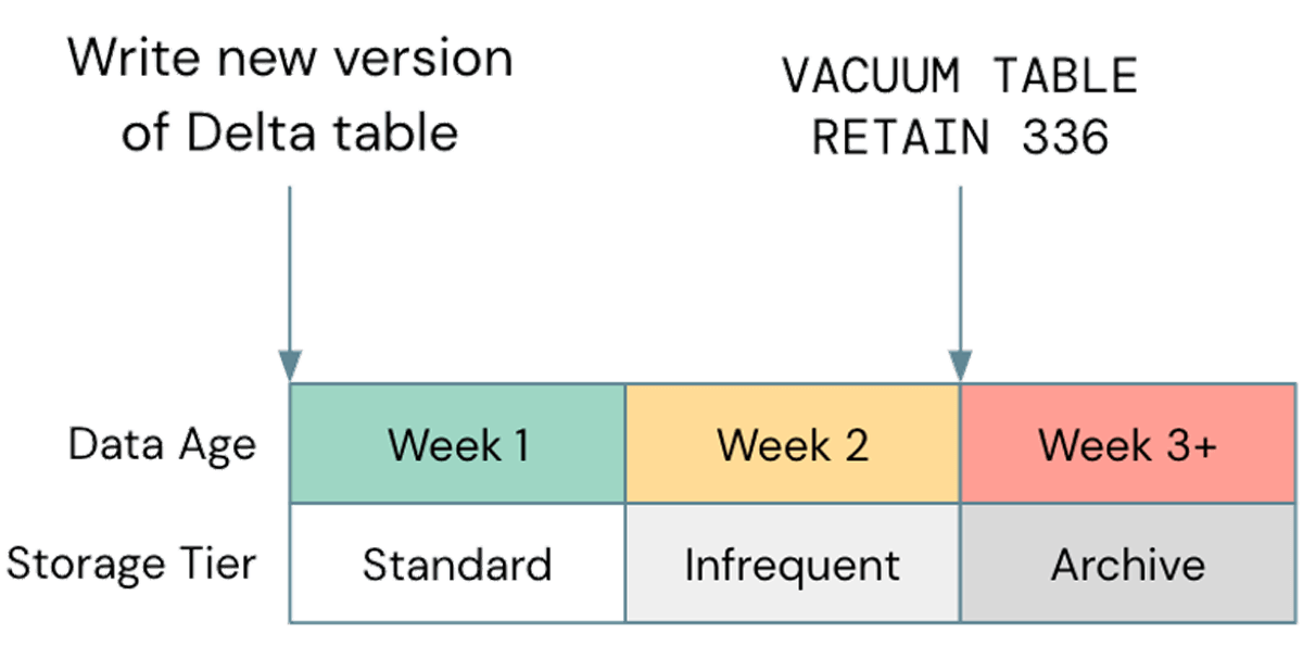
Note that non-standard storage tiers, such as Glacier on S3 or Archive on ADLS are not supported by Databricks, so be sure to Vacuum before those tiers are used.

Networking

Data used within the Databricks platform can come from a variety of different sources, from data warehouses to streaming systems like Kafka. However, the most common bandwidth utilizer is writing to storage layers such as S3 or ADLS. To reduce network costs, Databricks workspaces should be deployed with the goal of minimizing the amount of data being transferred between regions and availability zones. This includes deploying in the same region as the majority of your data where possible, and might include launching regional workspaces if necessary.

When using a customer-managed VPC for a Databricks workspace on AWS, networking costs can be reduced by leveraging VPC Endpoints which allow connectivity between the VPC and AWS services without an Internet Gateway or NAT Device. Using endpoints reduces the costs incurred from network traffic and also makes the connection more secure. Gateway endpoints specifically can be used for connecting to S3 and DynamoDB while interface endpoints can similarly be used to reduce the cost of compute instances connecting to the Databricks control plane. These endpoints are available as long as the workspace uses Secure Cluster Connectivity.

Similarly on Azure, Private Link or Service Endpoints can be configured for Databricks to communicate with services such as ADLS to reduce NAT costs. On GCP, Private Google Access (PGA) can be leveraged so that the traffic between Google Cloud Storage (GCS) and Google Container Registry (GCR) uses Google's internal network rather than the public internet, consequently also bypassing the use of a NAT device.

Serverless compute

For analytics workloads, an option to consider is to use a SQL Warehouse with the Serverless option enabled. With Serverless SQL, the Databricks platform manages a pool of compute instances that are ready to be assigned to a user whenever a workload is initiated. Therefore the costs of the underlying instances are fully managed by Databricks rather than having two separate charges (i.e. the DBU compute cost and the underlying cloud compute cost).

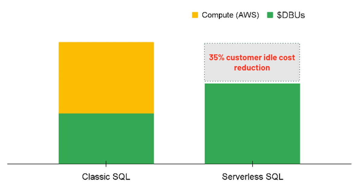
Serverless leads to a cost advantage by providing instant compute resources when a query is executed, reducing idle costs of underutilized clusters. In the same vein, serverless allows for more precise auto-scaling so that workloads can be efficiently completed, consequently saving on costs by improving performance. Though the serverless option is not yet directly enforceable through a policy, admins can enable the option for all users with SQL Warehouse creation permissions.

Monitoring usage

Along with controlling costs through cluster policies and workspace deployment configurations, it is equally important for admins to have the ability to monitor costs. Databricks provides a few options to do so with capabilities to automate notifications and alerts based on usage analytics. Specifically, administrators can use the Databricks account console for a quick usage overview, analyze usage logs for a more granular view, and use our new Budgets API to get active notifications when budgets are exceeded.

Using the account console

With the Databricks Enterprise 2.0 architecture the account console includes a usage page providing admins the ability to see usage by DBU or Dollar amount visually. The chart can show the consumption with an aggregated view, grouped by workspace, or grouped by SKUs. When grouping by SKUs the usage is shown by job clusters, all purpose clusters, or SQL compute as examples. If the chart is segmented by workspace, there will be a group shown for the top nine workspaces by DBU consumption with the last grouping as a combined sum of all the other workspaces. To understand the more granular details of every single workspace individually, a table can be found at the bottom of the page that lists out each workspace separately along with the DBU/$USD amounts by SKU. This page is well-suited for admins to get a full view of the usage and costs across all workspaces under an account.

As Databricks is a first party service on the Azure platform, the Azure Cost Management tool can be leveraged to monitor Databricks usage (along with all other services on Azure). Unlike the Account Console for Databricks deployments on AWS and GCP, the Azure monitoring capabilities provide data down to the tag granularity level. Custom tags on Azure can be created not only on the cluster level but also on the workspace level. These tags will be shown as groups and filters when analyzing the usage data. Within these reports, the usage generated by Databricks compute will be displayed along with the underlying instance usage conveniently within the same view. Logs can also be delivered to a storage container on a schedule and used for more automated analysis and alerts as explained in the next section.

Admins have the option to download usage logs manually from the account console usage page or with the Account API. However, a more efficient process for analyzing these usage logs is to configure automated log delivery to cloud storage (AWS, GCP). This results in a daily CSV which contains the usage for each workspace in a granular schema.

Once usage log delivery has been configured in any of the three clouds, a common best practice is to create a data pipeline within Databricks that will ingest this data daily and save it into a Delta table using a scheduled workflow. This data can then be used for usage analysis or to trigger alerts notifying admins or team leaders accountable for cost center spend when consumption reaches a set threshold.

Budgets API

One upcoming feature to make budgeting on Databricks compute costs easier is the new budget endpoint (currently in Private Preview) within the Account API. This will allow for anyone using a Databricks workspace to get notified once a budget threshold is hit on any custom timeframe filtered by workspace, SKU, or cluster tag. Hence, a budget can be configured for any workspace, cost center, or team through this API.

Summary

Although the Databricks Lakehouse Platform spans many use cases and user personas, we aim to provide a unified set of tools to help admins balance cost control with user experience. In this blog we laid out several strategies to approach this balance:

1. Use Cluster Policies to control which users are able to create clusters, as well as the size and scope of those clusters
2. Design your environment to minimize non-DBU costs generated by Databricks workspaces, such as storage and networking costs
3. Use monitoring tools in order to make sure your expectations of cost are being met and that you have effective practices in place

Check out our other admin-focused blogs linked throughout this article, and keep an eye out for additional blogs coming soon. Also be sure to try out new features such as Private Link (AWS | Azure) and Budgeting!