Introducing Real-Time Mode in Apache Spark™ Structured Streaming
Process events in milliseconds using Spark’s new Real-Time trigger
by Jerry Peng, Siying Dong, Abhay Bothra, Fatih Emekci, Karthikeyan Ramasamy, Navneeth Nair, Indrajit Roy, Matt Jones, Craig Lukasik and Ryan Nienhuis
- Stream processing in milliseconds: Spark Structured Streaming introduces real-time mode for processing data in milliseconds, enabling a new class of low-latency apps.
- No rewrites required: Teams can enable real-time mode with a simple config change - no replatforming or code overhauls needed.
- Now in Public Preview: Available on Databricks with support for popular sources and sinks; ideal for fraud detection, live personalization, and ML feature serving.
Apache Spark™ Structured Streaming has long powered mission-critical pipelines at scale, from streaming ETL to near real-time analytics and machine learning. Now, we’re expanding that capability to an entirely new class of workloads with real-time mode, a new trigger type that processes events as they arrive, with latency in the tens of milliseconds.
Unlike existing micro-batch triggers, which either process data on a fixed schedule (ProcessingTime trigger) or process all available data before shutting down (AvailableNow trigger), real-time mode continuously processes data and emits results as soon as they’re ready. This enables ultra-low-latency use cases like fraud detection, live personalization, and real-time machine learning feature serving, all without changing your existing code or replatforming.
This new mode is being contributed to open source Apache Spark and is now available in Public Preview on Databricks.
In this post, we’ll cover:
- What real-time mode is and how it works
- The types of applications it enables
- How you can start using it today
What is real-time mode?
Real-time mode delivers continuous, low-latency processing in Spark Structured Streaming, with p99 latencies as low as the single-digit milliseconds. Teams can enable it with a single configuration change — no rewrites or replatforming required — while keeping the same Structured Streaming APIs they use today.
How real-time mode works
Real-time mode runs long-lived streaming jobs that schedule stages concurrently. Data passes between tasks in memory using a streaming shuffle, which:
- Reduces coordination overhead
- Removes the fixed scheduling delays of micro-batch mode
- Delivers consistent sub-second performance
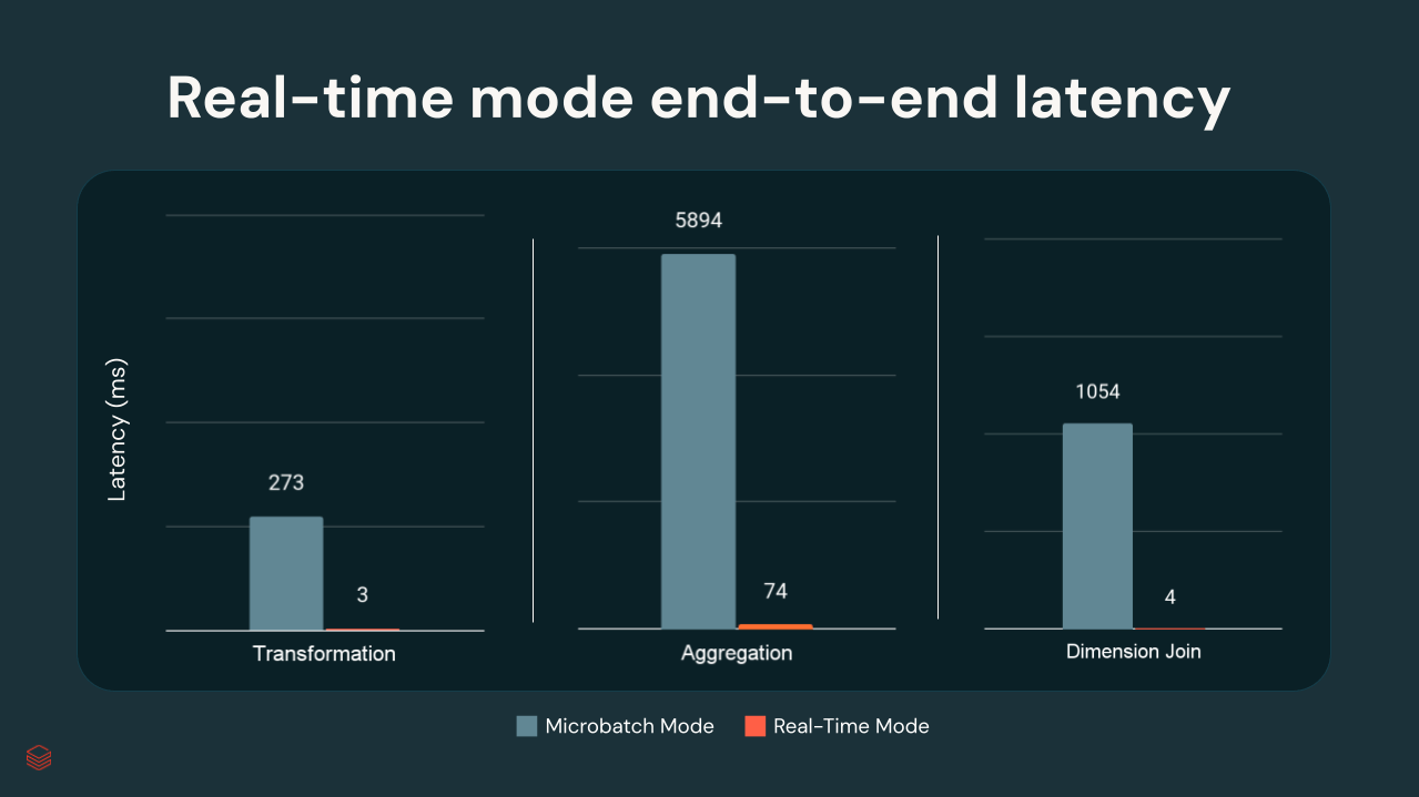
In Databricks internal tests, p99 latencies ranged from a few milliseconds to ~300 ms, depending on transformation complexity:
Applications and Use Cases
Real-time mode is designed for streaming applications that require ultra-low-latency processing and rapid response times, often in the critical path of business operations.
Real-Time Mode in Spark Structured Streaming has delivered remarkable results in our early testing. For a mission-critical payments authorization pipeline, where we perform encryption and other transformations, we achieved P99 end-to-end latency of just 15 milliseconds. We’re optimistic about scaling this low-latency processing across our data flows while consistently meeting strict SLAs. —Raja Kanchumarthi, Lead Data Engineer, Network International

In addition to Network International’s payment authorization use case quoted above, several early adopters have already used it to power a wide range of workloads:
Fraud detection in financial services: A global bank processes credit card transactions from Kafka in real time and flags suspicious activity, all within 200 milliseconds - reducing risk and response time without replatforming.
Personalized experiences in retail and media: An OTT streaming provider updates content recommendations immediately after a user finishes watching a show. A leading e-commerce platform recalculates product offers as customers browse - keeping engagement high with sub-second feedback loops.
Live session state and search history: A major travel site tracks and surfaces each user’s recent searches in real time across devices. Every new query updates the session cache instantly, enabling personalized results and autofill without delay.
Real-time ML Feature Serving: A food delivery app updates features like driver location and prep times in milliseconds. These updates flow directly into machine learning models and user-facing apps, improving ETA accuracy and customer experience.
These are just a few examples. Real-time mode can support any workload that benefits from turning data into decisions in milliseconds, from IoT sensor alerts and supply chain visibility to live gaming telemetry and in-app personalization.
Getting Started with real-time mode
Real-time mode is now available in Public Preview on Databricks. If you’re already using Structured Streaming, you can enable it with a single configuration and trigger update - no rewrites required.
To try it out in DBR 16.4 or above:
- Create a cluster (we recommend Dedicated Mode) on Databricks with Public Preview access.
Enable real-time mode by setting the following configuration:
Use the new trigger in your query:
Checkpointing
The trigger(RealTimeTrigger.apply(...)) option enables the new real-time execution mode, allowing you to achieve sub-second processing latencies. RealTimeTrigger accepts an argument that specifies how frequently the query checkpoints. For example, trigger(RealTimeTrigger.apply(“x minutes”)) By default, the checkpoint interval is 5 minutes, which works well for most use cases. Reducing this interval increases checkpoint frequency, but may impact latency. Most streaming sources and sinks are supported, including Kafka, Kinesis, and forEach for writing to external systems.
Summary
Real-time mode is ideal for use cases that demand the lowest possible latency. For many analytical workloads, standard micro-batch mode may be more cost-effective while still meeting latency requirements. Real-time mode introduces slight system overhead, so we recommend using it for latency-critical pipelines such as those examples above. Support for additional sources and sinks is expanding, and we’re actively working to broaden compatibility and further reduce latency.
For more details, please review the real-time mode documentation for full implementation details, supported sources and sinks, and example queries. You’ll find everything you need to enable the new trigger and configure your streaming workloads.
For a broader look at what's new in Apache Spark, including how real-time mode fits into the evolution of the engine, watch Michael Armbrust’s Spark keynote from DAIS 2025. It covers the architectural shifts behind Spark’s next chapter, with real-time mode as a core part of the story.
To go deeper on the engineering behind real-time mode, watch our engineers’ technical deep dive session, which walks through the design and implementation.
And to see how real-time mode fits into the broader streaming strategy on Databricks, check out the Comprehensive Guide to Streaming on the Data Intelligence Platform.
Get the latest posts in your inbox
Subscribe to our blog and get the latest posts delivered to your inbox.