Introduction to Databricks and PySpark for SAS Developers
by Ian J. Ghent, Bryan Chuinkam, Ban (Mike) Sun and Satish Garla
This is a collaborative post between Databricks and WiseWithData. We thank Founder and President Ian J. Ghent, Head of Pre-Sales Solutions R&D Bryan Chuinkam, and Head of Migration Solutions R&D Ban (Mike) Sun of WiseWithData for their contributions.
Technology has come a long way since the days of SAS®-driven data and analytics workloads. The lakehouse architecture is enabling data teams to process all types of data (structured, semi-structured and unstructured) for different use cases (data science, machine learning, real-time analytics, or classic business intelligence and data warehousing) all from a single copy of data. Performance and capabilities are combined with elegance and simplicity, creating a platform that is unmatched in the world today. Open-source technologies such as Python and Apache Spark™ have become the #1 language for data engineers and data scientists, in large part because they are simple and accessible.
Many SAS users are boldly embarking on modernizing their skill sets. While Databricks and PySpark are designed to be simple to learn, it can be a learning curve for experienced practitioners focused on SAS. But the good news for the SAS developer community is that Databricks embodies the concept of open and simple platform architecture and makes it easy for anyone who wants to build solutions in the modern data and AI cloud platform. This article surfaces some of the component mapping between the old and new world of analytics programming.
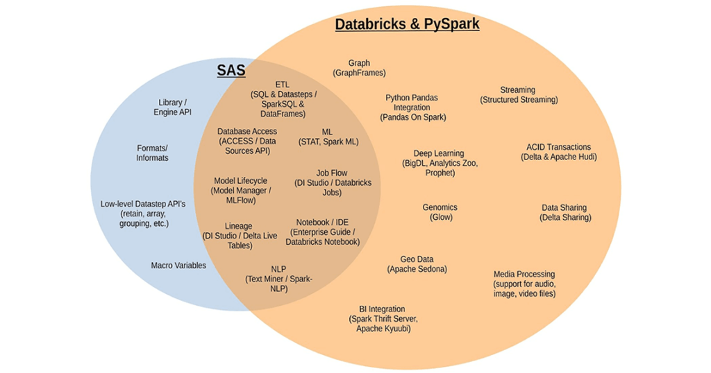
Finding a common ground
For all their differences, SAS and Databricks have some remarkable similarities. Both are designed from the ground up to be unified, enterprise grade platforms. They both let the developer mix and match between SQL and much more flexible programming paradigms. Both support built-in transformations and data summarization capabilities. Both support high-end analytical functions like linear and logistic regression, decision trees, random forests and clustering. They also both support a semantic data layer that abstracts away the details of the underlying data sources. Let’s do a deeper dive into some of these shared concepts.
SAS DATA steps vs DataFrames
The SAS DATA step is arguably the most powerful feature in the SAS language. You have the ability to union, join, filter and add, remove and modify columns, along with plainly express conditional and looping business logic. Proficient SAS developers leverage it to build massive DATA step pipelines to optimize their code and avoid I/O.
The PySpark DataFrame API has most of those same capabilities. For many use cases, DataFrame pipelines can express the same data processing pipeline in much the same way. Most importantly DataFrames are super fast and scalable, running in parallel across your cluster (without you needing to manage the parallelism).
| Example SAS Code | Example PySpark Code |
|---|---|
data df1;
    set df2;
    x = 1;
	run;
|
data df1;
    df1 = (
    df2
    .withColumn('x', lit(1))
)
|
SAS PROC SQL vs SparkSQL
The industry standard SQL is the lowest common denominator in analytics languages. Almost all tools support it to some degree. In SAS, you have a distinct tool that can use SQL, called PROC SQL and lets you interact with your SAS data sources in a way that is familiar to many who know nothing about SAS. It’s a bridge or a common language that almost everyone understands.
PySpark has similar capabilities, by simply calling spark.sql(), you can enter the SQL world. But with Apache Spark™, you have the ability to leverage your SQL knowledge and can go much further. The SQL expression syntax is supported in many places within the DataFrame API, making it much easier to learn. Another friendly tool for SQL programmers is Databricks SQL with an SQL programming editor to run SQL queries with blazing performance on the lakehouse.
| Example SAS Code | Example PySpark Code |
|---|---|
proc sql;
    create table sales_last_month as
    select
        customer_id
        ,sum(trans_amt) as sales_amount
    from sales.pos_sales
    group by customer_id
    order by customer_id;
quit;
|
sales['sales'].createOrReplaceTempView('sales')
work['sales_last_month'] = spark.sql("""
SELECT customer_id ,
       sum(trans_amt) AS sales_amount
FROM sales
GROUP BY customer_id
ORDER BY customer_id
""")
|
Base SAS Procs vs PySpark DataFrame transformations
SAS packages up much of its pre-built capabilities into procedures (PROCs). This includes transformations like data aggregation and summary statistics, as well as data reshaping, importing/exporting, etc. These PROCs represent distinct steps or process boundaries in a large job. In contrast, those same transformations in PySpark can be used anywhere, even within a DataFrame pipeline, giving the developer far more flexibility. Of course, you can still break them up into distinct steps.
| Example SAS Code | Example PySpark Code |
|---|---|
proc means data=df1 max min;
    var MSRP Invoice;
	where Make = 'Acura';
    output out = df2;
run;
|
df2 = (
    df1.filter("Make = 'Acura'")
    .select("MSRP", "Invoice")
    .summary('max','min')
)
|
Lazy execution – SAS “run” statement vs PySpark actions
The lazy execution model in Spark is the foundation of so many optimizations, which enables PySpark to be so much faster than SAS. Believe it or not, SAS also has support for lazy execution! Impressive for a language designed over 50 years ago. You know all those “run” (and “quit”) statements you are forced to write in SAS? They are actually its own version of PySpark actions.
In SAS, you can define several steps in a process, but they don’t execute until the “run” is called. The main difference between SAS and PySpark is not the lazy execution, but the optimizations that are enabled by it. In SAS, unfortunately, the execution engine is also “lazy,” ignoring all the potential optimizations. For this reason, lazy execution in SAS code is rarely used, because it doesn’t help performance.
So the next time you are confused by the lazy execution model in PySpark, just remember that SAS is the same, it’s just that nobody uses the feature. Your Actions in PySpark are like the run statements in SAS. In fact, if you want to trigger immediate execution in PySpark (and store intermediate results to disk), just like the run statement, there’s an Action for that. Just call “.checkpoint()” on your DataFrame.
| Example SAS Code | Example PySpark Code |
|---|---|
data df1;
    set df2;
    x = 1;
run;
|
df1 = (
    df2
    .withColumn('x', lit(1))
).checkpoint()
|
Advanced analytics and Spark ML
Over the past 45 years, the SAS language has amassed some significant capabilities for statistics and machine learning. The SAS/STAT procedures package up vast amounts of capabilities within their odd and inconsistent syntax. On the other-hand, SparkML includes capabilities that cover much of the modern use cases for STAT, but in a more cohesive and consistent way.
One notable difference between these two packages is the overall approach to telemetry and diagnostics. With SAS, you get a complete dump of every and all statistical measures when you do a machine learning task. This can be confusing and inefficient for modern data scientists.
Typically, data scientists only need one or a small set of model diagnostics they like to use to assess their model. That’s why SparkML takes a different and more modular approach by providing APIs that let you get those diagnostics on request. For large data sets, this difference in approach can have significant performance implications by avoiding computing statistics that have no use.
It’s also worth noting that everything that’s in the PySpark ML library are parallelized algorithms, so they are much faster. For those purists out there, yes we know a single-threaded logistic regression model will have a slightly better fit. We’ve all heard that argument, but you’re totally missing the point here. Faster model development means more iterations and more experimentation, which leads to much better models.
| Example SAS Code | Example PySpark Code |
|---|---|
proc logistic data=ingots; model NotReady = Heat Soak; run; |
vector_assembler = VectorAssembler(inputCols=['Heat', 'Soak'], outputCol='features')
v_df = vector_assembler.transform(ingots).select(['features', 'NotReady'])
lr = LogisticRegression(featuresCol='features', labelCol='NotReady')
lr_model = lr.fit(v_df)
lr_predictions = lr_model.transform(v_df)
lr_evaluator = BinaryClassificationEvaluator(
    rawPredictionCol='rawPrediction', labelCol='NotReady')
print('Area Under ROC', lr_evaluator.evaluate(lr_predictions))
|
In the PySpark example above, the input columns “Heat, Soak” are combined into a single feature vector using the VectorAssembler API. A logistic regression model is then trained on the transformed data frame using the LogisticRegression algorithm from SparkML library. To print the AUC metric,the BinaryClassificationEvaluator is used with predictions from the trained model and the actual label as inputs. This modular approach gives better control in calculating the model performance metrics of choice.
The differences
While there are many commonalities between SAS and PySpark, there are also a lot of differences. As a SAS expert learning PySpark, some of these differences can be very difficult to navigate. Let’s break them into a few different categories. There are some SAS features that aren’t available natively in PySpark, and then there are things that just require a different tool or approach in PySpark.
Different ecosystem
The SAS platform is a whole collection of acquired and internally developed products, many of which work relatively well together. Databricks is built on open standards, as such, you can easily integrate thousands of tools. Let’s take a look at some SAS-based tools and capabilities available in Databricks for similar use cases.
Let’s start with SAS® Data Integration Studio (DI Studio). Powered by a complicated metadata driven model, DI Studio fills some important roles in the SAS ecosystem. It primarily provides a production job flow orchestration capability for ETL workloads. In Databricks, data engineering pipelines are developed and deployed using Notebooks and Jobs. Data engineering tasks are powered by Apache Spark (the de-facto industry standard for big data ETL).
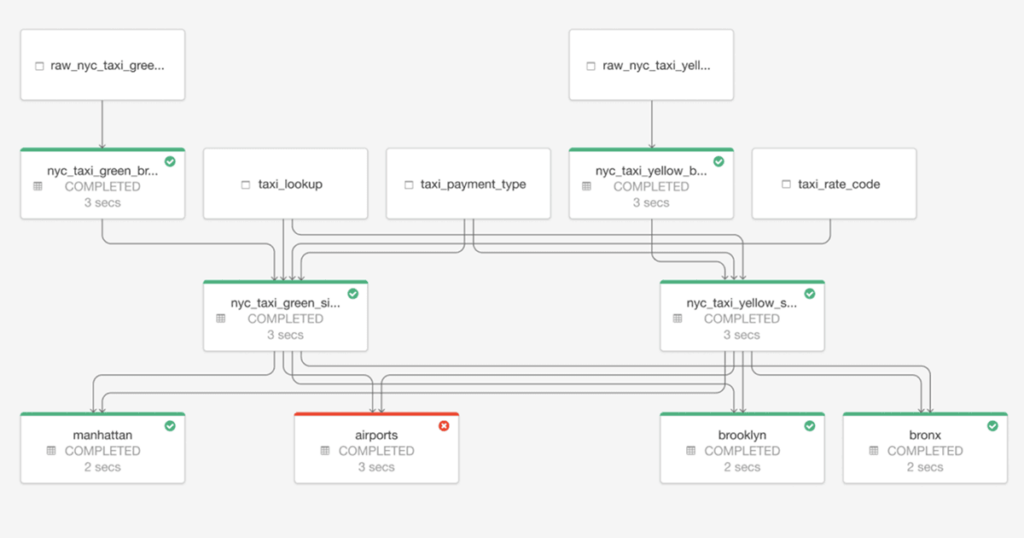
Databricks’ Delta Live Tables(DLT) and Job orchestrations further simplifies ETL pipeline development on the Lakehouse architecture. DLT provides a reliable framework to declaratively create ETL pipelines instead of traditional procedural sequence of transformation. Meaning, the user describes the desired results of the pipeline without explicitly listing the ordered steps that must be performed to arrive at the result. DLT engine intelligently figures out “how” the compute framework should carry out these processes.
The other key role that DI Studio plays is to provide data lineage tracking. This feature, however, only works properly when you set everything up just right and manually input metadata on all code nodes (a very painful process). In contrast, DLT ensures that the generated pipeline automatically captures the dependency between datasets, which is used to determine the execution order when performing an update and recording lineage information in the event log for a pipeline.
While most data scientists are very happy coders, some prefer point-and-click data mining tools. There’s an emerging term for these folks, called “citizen data scientists,” whose persona is analytical, but not deeply technical. In SAS, you have the very expensive tool SAS® Enterprise Miner to build models without coding. This tool, with its user interface from a bygone era, lets users sample, explore, modify, model and assess their SAS data all from the comfort of their mouse, no keyboard required. Another point and click tool in SAS, called SAS® Enterprise Guide, is the most popular interface to both SAS programming and point-and-click analysis. Because of SAS’ complex syntax, many people like to leverage the point-and-click tools to generate SAS code that they then modify to suit their needs.
With PySpark, the APIs are simpler and more consistent, so the need for helper tools is reduced. Of course the modern way to do data science is via notebooks, and the Databricks notebook does a great job at doing away with coding for tasks that should be point and click, like graphing out your data. Exploratory analysis of data and model development in Databricks is performed using Databricks ML Runtime from Databricks Notebooks. With Databricks AutoML, users are provided a point-n-click option to quickly train and deploy a model. Databricks AutoML takes a “glass-box” approach by generating editable, shareable notebooks with baseline models that integrate with MLflow Tracking and best practices to provide a modifiable starting point for new projects.
With the latest acquisition of 8080 Labs, a new capability that will be coming to Databricks notebooks and workspace is performing data exploration and analytics using low code/no-code. The bamboolib package from 8080 Labs automatically generates Python code for user actions performed via point-n-click.
Putting it all together, Lakehouse architecture powered by open source Delta Lake in Databricks simplifies data architectures and enables storing all your data once in a data lake and doing AI and BI on that data directly.
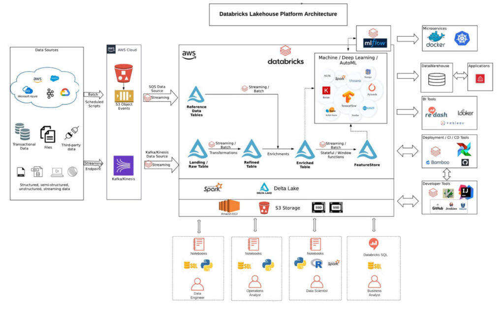
The diagram above shows a reference architecture of Databricks deployed on AWS (the architecture will be similar on other cloud platforms) supporting different data sources, use cases and user personas all through one unified platform. Data engineers get to easily use open file formats such as Apache Parquet, ORC along with in-built performance optimization, transaction support, schema enforcement and governance.
Data engineers now have to do less plumbing work and focus on core data transformations for using streaming data with built in structured streaming and Delta Lake tables. ML is a first-class citizen in the lakehouse, which means data scientists do not waste time subsampling or moving data to share dashboards. Data and operational analysts can work off the same data layer as other data stakeholders and use their beloved SQL programming language to analyze data.
Different approaches
As with all changes, there are some things you just need to adapt. While much of the functionality of SAS programming exists in PySpark, some features are meant to be used in a totally different way. Here are a few examples of the types of differences that you’ll need to adapt to, in order to be effective in PySpark.
Procedural SAS vs Object Oriented PySpark
In SAS, most of your code will end up as either a DATA step or a procedure. In both cases, you need to always explicitly declare the input and output datasets being used (i.e. data=dataset). In contrast, PySpark DataFrames use an object oriented approach, where the DataFrame reference is attached to the methods that can be performed on it. In most cases, this approach is far more convenient and more compatible with modern programming techniques. But, it can take some getting used to, especially for developers that have never done any object-oriented programming.
| Example SAS Code | Example PySpark Code |
|---|---|
proc sort data=df1 out=dedup nodupkey; by cid; run; |
dedup=df1.dropDuplicates(['cid']).orderBy(['cid']) |
Data reshaping
Let’s take, for example, the common task of data reshaping in SAS, notionally having “proc transpose.” Transpose, unfortunately, is severely limited because it’s limited to a single data series. That means for practical applications you have to call it many times and glue the data back together. That may be an acceptable practice on a small SAS dataset, but it could cause hours of additional processing on a larger dataset. Because of this limitation, many SAS developers have developed their own data reshaping techniques, many using some combination of DATA steps with retain, arrays and macro loops. This reshaping code often ends up being 100’s of lines of SAS code, but is the most efficient way to execute the transformation in SAS.
Many of the low-level operations that can be performed in a DATA step are just not available in PySpark. Instead, PySpark provides much simpler interfaces for common tasks like data reshaping with the groupBy().pivot() transformation, which supports multiple data series simultaneously.
| Example SAS Code | Example PySpark Code |
|---|---|
proc transpose data=test out=xposed; by var1 var2; var x; id y; run |
xposed = (test
    .groupBy('var1','var2')
    .pivot('y')
    .agg(last('x'))
    .withColumn('_name_',lit('y'))
)
|
Column oriented vs. business-logic oriented
In most data processing systems, including PySpark, you define business-logic within the context of a single column. SAS by contrast has more flexibility. You can define large blocks of business-logic within a DATA step and define column values within that business-logic framing. While this approach is more expressive and flexible, it can also be problematic to debug.
Changing your mindset to be column oriented isn’t that challenging, but it does take some time. If you are proficient in SQL, it should come pretty easily. What’s more problematic is adapting existing business-logic code into a column-oriented world. Some DATA steps contain thousands of lines of business-logic oriented code, making manual translation a complete nightmare.
| Example SAS Code | Example PySpark Code |
|---|---|
data output_df;
    set input_df;
    if x = 5 then do;
        a = 5;
        b = 6;
        c = 7;
    end;
    else if x = 10 then do;
        a = 10;
        b = 11;
        c = 12;
    end;
    else do;
        a = 1;
        b = -1;
        c = 0;
    end;
run;
|
output_df = (
    input_df
    .withColumn('a', expr("""case
        when (x = 5) then 5
        when (x = 10) then 10
        else 1 end"""))
    .withColumn('b', expr("""case
        when (x = 5) then 6
        when (x = 10) then 11
        else -1 end"""))
    .withColumn('c', expr("""case
        when (x = 5) then 7
        when (x = 10) then 12
        else 0 end"""))
)
|
The missing features
There are a number of powerful and important features in SAS that just don’t exist in PySpark. When you have your favorite tool in the toolbox, and suddenly it's missing, it doesn’t matter how fancy or powerful the new tools are; that trusty Japanese Dozuki saw is still the only tool for some jobs. In modernizing with PySpark, you will indeed encounter these missing tools that you are used to, but don’t fret, read on and we’ve got some good news. First let’s talk about what they are and why they’re important.
Advanced SAS DATA step features
Let’s say you want to generate new rows conditionally, keep the results from previous rows calculations or create totals and subtotals with embedded conditional logic. These are all tasks that are relatively simple in our iterative SAS DATA step API, but our trusty PySpark DataFrame is just not equipped to easily handle.
Some data processing tasks need to have complete fine-grained control over the whole process, in a “row iterative” manner. Such tasks aren’t compatible with PySpark’s shared-nothing MPP architecture, which assumes rows can be processed completely independently of each other. There are only limited APIs like the window function to deal with inter-row dependencies. Finding solutions to these problems in PySpark can be very frustrating and time consuming.
| Example SAS Code |
|---|
data df2;
    set df;
    by customer_id seq_num;
    retain counter;
    label = "     ";
    if first.customer_id then counter = 0;
    else counter = counter+1;
    output;
    if last.customer_id then do;
        seq_num = .;
        label = "Total";
        output;
    end;
run;
|
Custom formats and informats
SAS formats are remarkable in their simplicity and usefulness. They provide a mechanism to reformat, remap and represent your data in one tool. While the built-in formats are useful for handling common tasks such as outputting a date string, they are also useful for numeric and string contexts. There are similar tools available in PySpark for these use cases.
The concept of custom formats or informats is a different story. They support both a simple mapping of key-value pairs, but also a mapping by range and support default values. While some use cases can be worked around by using joins, the convenience and concise syntax formats provided by SAS isn’t something that is available in PySpark.
| Example SAS Code |
|---|
proc format;
value prodcd
    1='Shoes'
2='Boots'
    3='Sandals'
;
run;
data sales_orders;
    set sales_orders;
    product_desc = put(product_code, prodcd.);
run;
|
The library concept & access engines
One of the most common complaints from SAS developers using PySpark is that it lacks a semantic data layer integrated directly into the core end-user API (i.e. Python session). The SAS data library concept is so familiar and ingrained, it’s hard to navigate without it. There’s the relatively new Catalog API in PySpark, but that requires constant calling back to the store and getting access to what you want. There’s not a way to just define a logical data store and get back DataFrame objects for each and every table all at once. Most SAS developers switching to PySpark don’t like having to call spark.read.jdbc to access each Database table, they are used to the access engine library concept, where all the tables in a database are at your fingertips.
| Example SAS Code |
|---|
libname lib1 ‘path1’;
libname lib2 ‘path2’;
data lib2.dataset;
    set lib1.dataset;
run;
|
Solving for the differences – the SPROCKET Runtime
While many of SAS language concepts are no longer relevant or handy, the missing features we just discussed are indeed very useful, and in some cases almost impossible to live without. That’s why WiseWithData has developed a special plugin to Databricks and PySpark that brings those familiar and powerful features into the modern platform, the SPROCKET Runtime. It’s a key part of how WiseWithData is able to automatically migrate SAS code into Databricks and PySpark at incredible speeds, while providing a 1-to-1 code conversion experience.
The SPROCKET libraries & database access engines
SPROCKET libraries let you fast track your analytics with a simplified way to access your data sources, just like SAS language libraries concept. This powerful SPROCKET Runtime feature means no more messing about with data paths and JDBC connectors, and access to all your data in a single line of code. Simply register a library and have all the relevant DataFrames ready to go.
| SAS | SPROCKET |
|---|---|
libname lib ‘path’; lib.dataset |
register_library(‘lib’, ‘path’) lib[‘dataset’] |
Custom formats / informats
With the SPROCKET Runtime, you can leverage the power & simplicity of custom Formats & Informats to transform your data. Transform your data inside PySpark DataFrames using custom formats just like you did in your SAS environment.
| SAS | SPROCKET |
|---|---|
proc format;
value prodcd
    1='Shoes'
    2='Boots'
    3='Sandals'
;
run;
data sales_orders;
    set sales_orders;
    product_desc = put(product_code, prodcd.);
run;
|
value_formats = [
    {'fmtname': 'prodcd', 'fmttype': 'N', 'fmtvalues': [
        {'start': 1, 'label': 'Shoes'},
        {'start': 2, 'label': 'Boots'},
        {'start': 3, 'label': 'Sandals'},
    ]}]
register_formats(spark, 'work', value_formats)
work['sales_orders'] = (
    work['sales_orders']
    .transform(put_custom_format(
        'product_desc', 'product_code', ‘prodcd'))
)
|
Macro variables
Macro variables are a powerful concept in the SAS language. While there are some similar concepts in PySpark, it’s just not the same thing. That’s why we’ve brought this concept into our SPROCKET Runtime, making it easy to use those concepts in PySpark.
| SAS | SPROCKET |
|---|---|
%let x=1; &x “value_&x._1” |
set_smv(‘x’, 1)
get_smv(‘x’)
“value_{x}_1”.format(**get_smvs())
|
Advanced SAS DATA step and the Row Iterative Processing Language (RIPL API)
The flexibility of the SAS DATA step language is available as a PySpark API within the SPROCKET Runtime. Want to use by-group processing, retained columns, do loops, and arrays? The RIPL API is your best friend. The RIPL API brings back the familiar business-logic-oriented data processing view. Now you can express business logic in familiar if/else conditional blocks in Python. All the features you know and love, but with the ease of Python and the performance and scalability of PySpark.
| SAS | SPROCKET – RIPL API |
|---|---|
data df2;
    set df;
    by customer_id seq_num;
    retain counter;
    label = "     ";
    if first.customer_id then counter = 0;
    else counter = counter+1;
    output;
    if last.customer_id then do;
        seq_num = .;
        label = "Total";
        output;
    end;
run;
|
def ripl_logic():
    rdv['label'] = '     '
    if rdv['_first_customer_id'] > 0:
        rdv['counter'] = 0
    else:
 rdv['counter'] = rdv['counter']+1
        output()
    if rdv['_last_customer_id'] > 0:
        rdv['seq_num'] = ripl_missing_num
        rdv['label'] = 'Total'
        output()

work['df2'] = (
    work['df']
        .transform(ripl_transform(
            by_cols=['customer_id', 'seq_num'],
            retain_cols=['counter'])
 )
|
Retraining is always hard, but we’re here to help
This journey toward a successful migration can be confusing, even frustrating. But you’re not alone, thousands of SAS-based professionals are joining this worthwhile journey with you. WiseWithData and Databricks are here to support you with tools, resources and helpful hints to make the process easier.
Try the course, Databricks for SAS Users, on Databricks Academy to get a basic hands-on experience with PySpark programming for SAS programming language constructs and contact us to learn more about how we can assist your SAS team to onboard their ETL workloads to Databricks and enable best practices.
SAS® and all other SAS Institute Inc. product or service names are registered trademarks or trademarks of SAS Institute Inc. in the USA and other countries. ® indicates USA registration.
Get the latest posts in your inbox
Subscribe to our blog and get the latest posts delivered to your inbox.