Building a Similarity-based Image Recommendation System for e-Commerce

Why recommendation systems are important

Online shopping has become the default experience for the average consumer – even established brick-and-mortar retailers have embraced e-commerce. To ensure a smooth user experience, multiple factors need to be considered for e-commerce. One core functionality that has proven to improve the user experience and, consequently revenue for online retailers, is a product recommendation system. In this day and age, it would be nearly impossible to go to a website for shoppers and not see product recommendations.

But not all recommenders are created equal, nor should they be. Different shopping experiences require different data to make recommendations. Engaging the shopper with a personalized experience requires multiple modalities of data and recommendation methods. Most recommenders concern themselves with training machine learning models on user and product attribute data massaged to a tabular form.

There has been an exponential increase in the volume and variety of data at our disposal to build recommenders and notable advances in compute and algorithms to utilize in the process. Particularly, the means to store, process and learn from image data has dramatically increased in the past several years. This allows retailers to go beyond simple collaborative filtering algorithms and utilize more complex methods, such as image classification and deep convolutional neural networks, that can take into account the visual similarity of items as an input for making recommendations. This is especially important given online shopping is a largely visual experience and many consumer goods are judged on aesthetics.

In this article, we’ll change the script and show the end-to-end process for training and deploying an image-based similarity model that can serve as the foundation for a recommender system. Furthermore, we’ll show how the underlying distributed compute available in Databricks can help scale the training process and how foundational components of the Lakehouse, Delta Lake and MLflow, can make this process simple and reproducible.

Why similarity learning?

Similarity models are trained using contrastive learning. In contrastive learning, the goal is to make the machine learning (ML) model learn an embedding space where the distance between similar items is minimized and the distance between dissimilar items is maximized. Here, we will use the fashion MNIST dataset, which comprises around 70,000 images of various clothing items. Based on the above description, a similarity model trained on this labeled dataset will learn an embedding space where embeddings of similar products (e.g., boots, are closer together and different items e.g., boots and pullovers) are far apart. In supervised contrastive learning, the algorithm has access to metadata, such as image labels, to learn from, in addition to the raw pixel data itself.

This could be illustrated as follows.

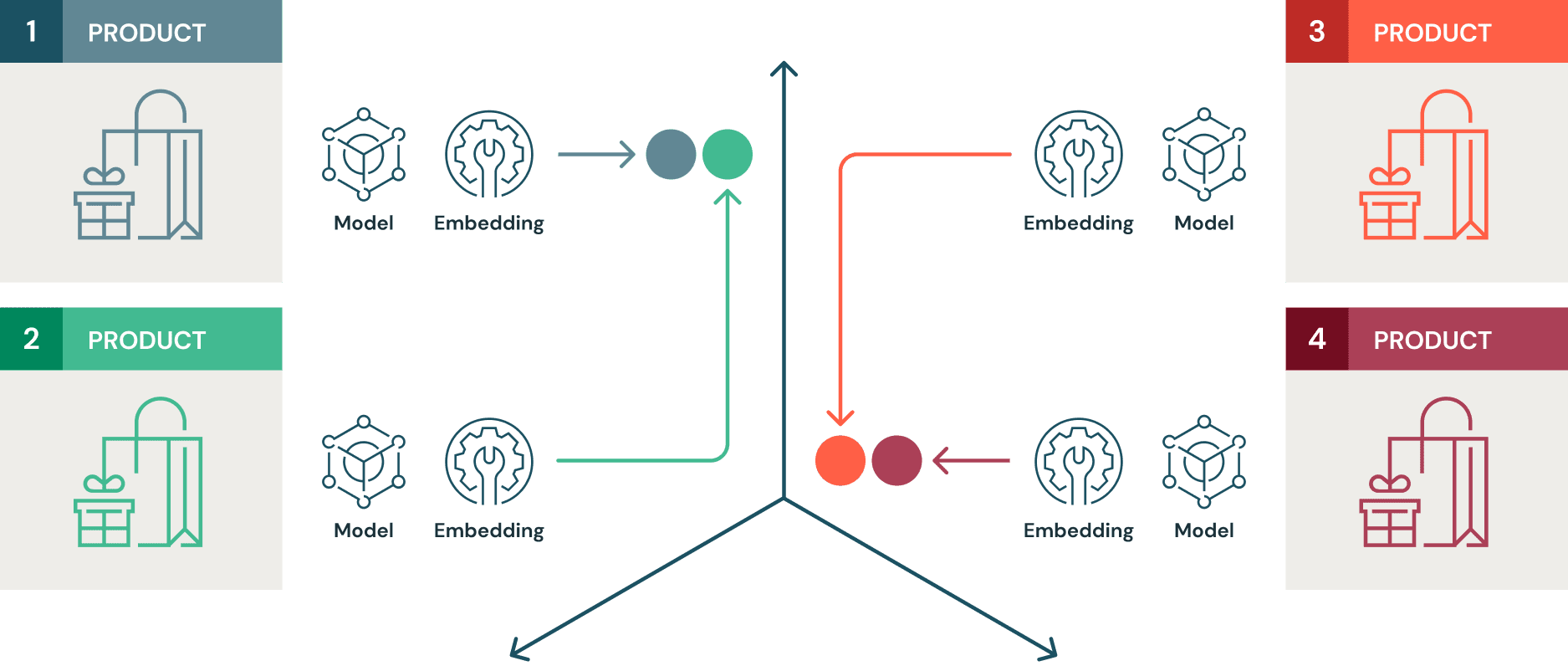
Traditional ML models for image classification focus on reducing a loss function that’s geared towards maximizing predicted class probabilities. However, what a recommender system fundamentally attempts to do to suggest alternatives to a given item. These items could be described as closer to one another in a certain embedding space than others. Thus, in most cases, the operating principle of recommendation systems closely align with that of contrastive learning mechanisms compared to traditional supervised learning. Furthermore, similarity models are more adept at generalizing to unseen data, based on their similarities. For example, if the original training data does not contain any images of jackets but contains images of hoodies and boots, a similarity model trained on this data would locate the embeddings of the image of a jacket closer to hoodies and farther away from boots. This is very powerful in the world of recommendation methods.

Specifically, we use the Tensorflow Similarity library to train the model and Apache Spark, combined with Horovod to scale the model training across a GPU cluster. We use Hyperopt to scale hyperparameter search across the GPU cluster with Spark in only a few lines of code. All these experiments will be tracked and logged with MLflow to preserve model lineage and reproducibility. Delta will be used as the data source format to track data lineage.

Setting up the environment

The supervised_hello_world example in the Tensorflow Similarity Github repository gives a perfect template to use for the task at hand. What we try to do with a recommender is similar to the manner in which a similarity model behaves. That is, you choose an image of an item, and you query the model to return n of the most similar items that could also pique your interest.

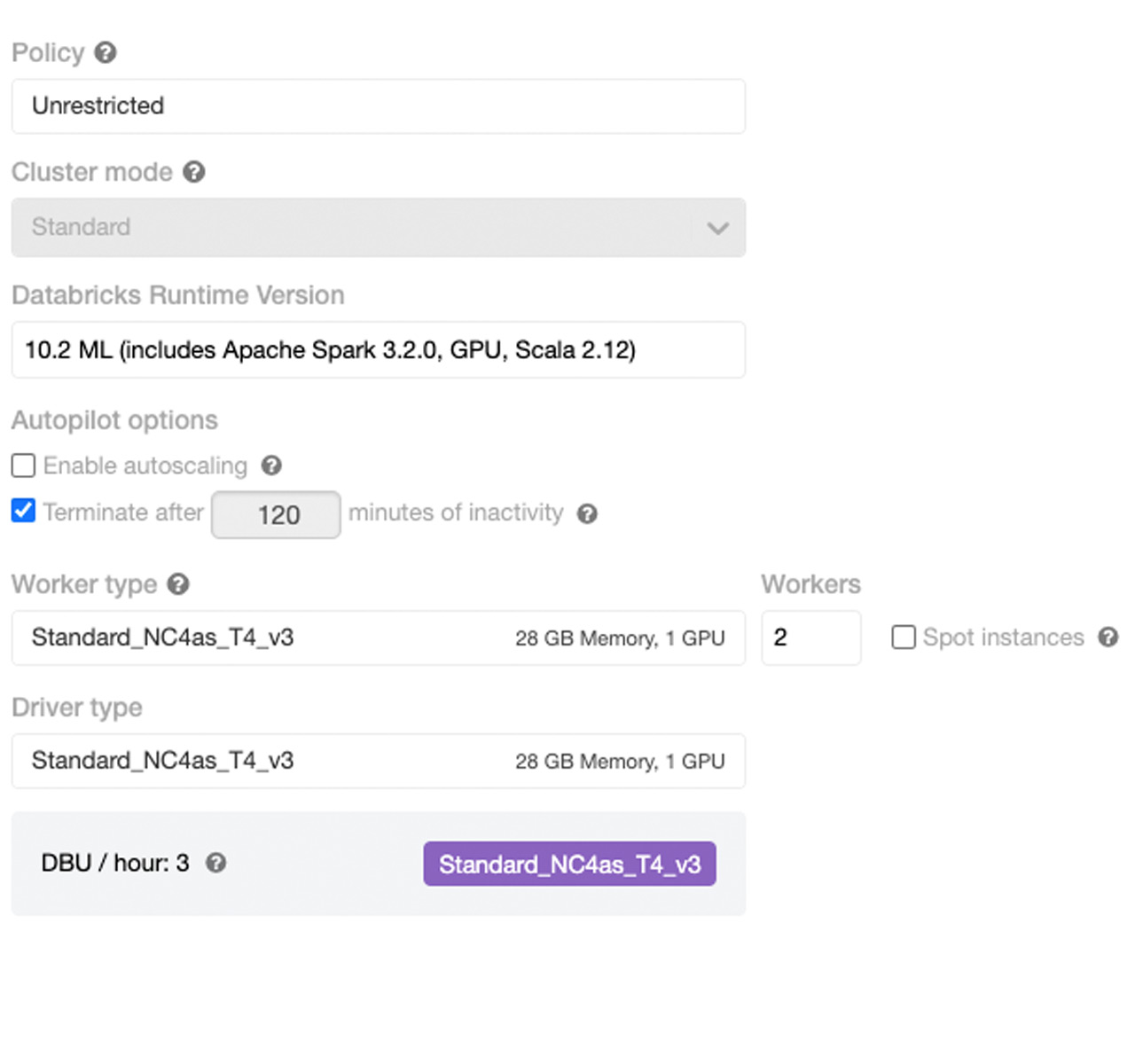
To fully leverage the Databricks platform, it’s best to spin up a cluster with a GPU node for the driver (since we will be doing some single node training initially), two or more GPU worker nodes (as we will be scaling hyperparameter optimization and distributing the training itself), and a Databricks Machine Learning runtime of 10.0 or above. T4 GPU instances are a good choice for this exercise.

The entire process should take no more than 5 minutes (including the cluster spin up time).

Ingest data into Delta tables

Fashion MNIST training and test data can be imported to our environment using a sequence of simple shell commands and the helper function `convert` (modified from the original version at: ‘https://pjreddie.com/projects/mnist-in-csv/’ (to reduce unnecessary file I/O) can be used to convert the image and label files into a tabular format. Subsequently these tables can be stored as Delta tables.

Storing the training and test data as Delta tables is important as we incrementally write new observations (new images and their labels) to these tables, the Delta transaction log can keep track of the changes to data. This enables us to track the fresh data we can use to re-index data in the similarity index we will describe later.

Nuances of training similarity models

A neural network used to train a similarity model is quite similar to one used for regular supervised learning. The primary differences here are in the loss function we use and the metric embedding layer. Here we use a simple convolutional neural network (cnn) architecture, which is commonly seen in computer vision applications. However, there are subtle differences in the code that enable the model to learn using contrastive methods.

You will see the multi similarity loss function in place of the softmax loss function for multiclass classification you would see otherwise. Compared to other traditional loss functions used for contrastive learning, Multi-Similarity Loss takes into account multiple similarities. These similarities are self similarity, positive relative similarity, and negative relative similarity. Multi-similarity Loss measures these three similarities by means of iterative hard pair mining and weighting, bringing significant performance gains in contrastive learning tasks. Further details of this specific loss is discussed at length in the original publication by Wang et al.

In the context of this example, this loss helps minimize the distance between similar items and maximize distance between dissimilar items in the embedding space. As explained in the supervised_hello_world example in the Tensorflow_Similarity repository, the embedding layer added to the model with the MetricEmbedding() is a dense layer with L2 normalization. For each minibatch, a fixed number of embeddings (corresponding to images) are randomly chosen from randomly sampled classes (the number of classes is a hyper parameter). These are then subjected to hard pair mining and weighting iteratively in the Multi-Similarity Loss layer, where information from three different types of similarities is used to penalize dissimilar samples in close proximity more.

This can be seen below.

```
def get_model():
    from tensorflow_similarity.layers import MetricEmbedding
    from tensorflow.keras import layers
    from tensorflow_similarity.models import SimilarityModel
    
    inputs = layers.Input(shape=(28, 28, 1))
    x = layers.experimental.preprocessing.Rescaling(1/255)(inputs)
    x = layers.Conv2D(32, 3, activation='relu')(x)
    x = layers.MaxPool2D(2, 2)(x)
    x = layers.Dropout(0.3)(x)
          …
          …
    x = layers.Dropout(0.3)(x)
    x = layers.Flatten()(x)
    outputs = MetricEmbedding(128)(x)
    return SimilarityModel(inputs, outputs)
…

…
loss = MultiSimilarityLoss(distance=distance)
model.compile(optimizer=Adam(learning_rate), loss=loss)

```

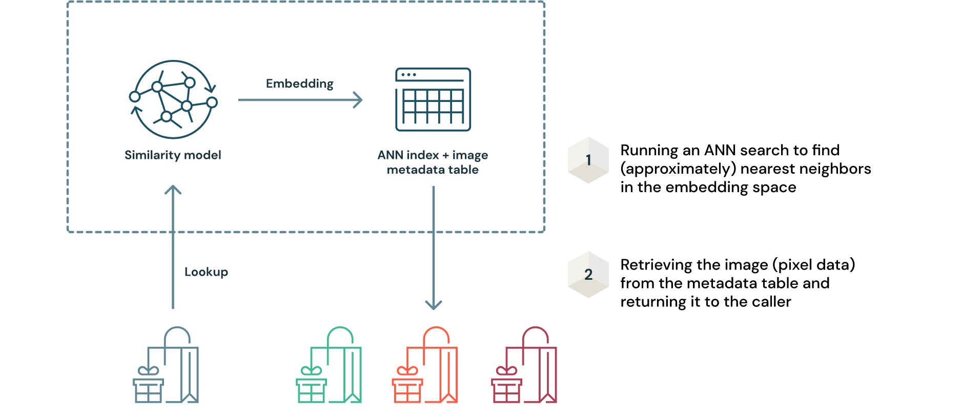
It is important to understand how a trained similarity model functions in TensorFlow Similarity. During training of the model, we learned embeddings that minimize the distance between similar items. The Indexer class of the library provides the capability to build an index from these embeddings on the basis of the chosen distance metric. For example, if the chosen distance metric is ‘cosine’, the index will be built on the basis of cosine similarity.

The index exists to quickly find items with ‘close’ embeddings. For this search to be quick, the most similar items have to be retrieved with relatively low latency. The query method here uses Fast Approximate Nearest Neighbor Search to retrieve the n nearest neighbors to a given item, which we can then serve as recommendations.

```
#Build an index using training data 
x_index, y_index = select_examples(x_train, y_train, CLASSES, 20)
tfsim_model.reset_index()
tfsim_model.index(x_index, y_index, data=x_index)

#Query the index using the lookup method
tfsim_model.lookup(x_display, k=5)
.
.
.
```

Leveraging parallelism with Apache Spark

This model can be trained in a single node without an issue and we can build an index to query it. Subsequently the trained model can be deployed to be queried via a REST endpoint with the help of MLflow. This particularly makes sense, since the fashion MNIST dataset used in this example is small and fits in a single GPU enabled instance’s memory easily. However, in practice, image datasets of products can span several gigabytes in size. Also, even for a model trained on a small dataset, the process of finding the optimal hyperparameters of the model can be a very time consuming process if done on a single GPU enabled instance. In both cases, parallelism enabled by Spark can do wonders only by changing a few lines of code.

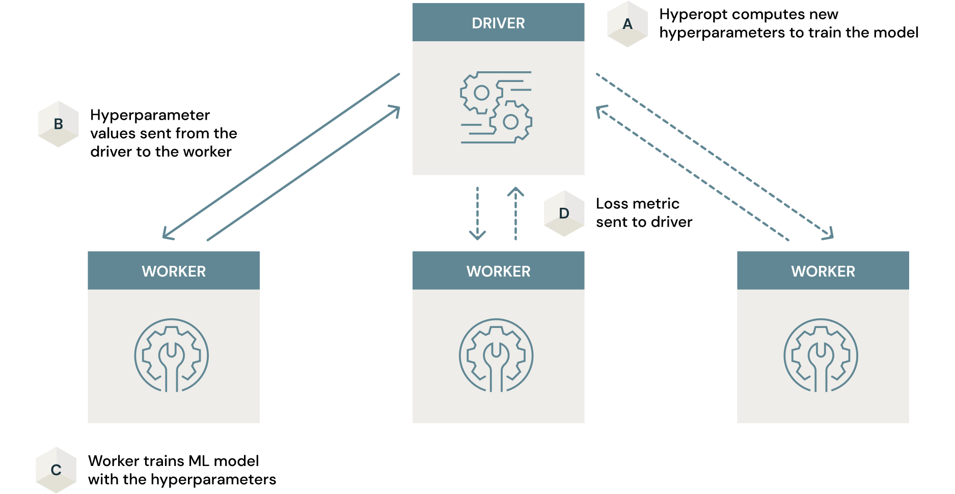
Parallelizing hyperparameter optimization with Apache Spark

In the case of a neural network, you could think of weights of the artificial neurons as parameters that are updated during training. This is performed by means of gradient descent and backpropagation of error. However, values such as the number of layers, the number of neurons per layer, and even the activation functions in neurons aren’t optimized during this process. These are termed hyperparameters, and we have to search the space of all such possible hyperparameter combinations in a clever way to proceed with the modeling process.

Traditional model tuning (a shorthand for hyperparameter search) can be done with naive approaches such as an exhaustive grid search or a random search. Hyperopt, a widely adopted open-source framework for model tuning, leverages far more efficient Bayesian search for this process.

This search can be time consuming, even with intelligent algorithms such as Bayesian search. However, Spark can work in conjunction with Hyperopt to parallelize this process across the entire cluster resulting in a dramatic reduction in the time consumed. All that has to be done to perform this scaling is to add 2 lines of python code to what you would normally use with Hyepropt. Note how the parallelism argument is set to 2, (i.e. the number of cluster GPUs).

```
.
.
from hyperopt import SparkTrials
.
.
trials = SparkTrials(parallelism = 2)
.
.
best_params = fmin(
    fn=train_hyperopt,
    space=space,
    algo=algo,
    max_evals=32,
    trials = trials
  )
.
.

```

The mechanism in which this parallelism works can be illustrated as follows.

The article Scaling Hyperopt to Tune Machine Learning Models in Python gives an excellent deep dive on how this works. It is important to use GPU enabled nodes for this process in the case of similarity models, particularly in this example leveraging Tensorflow. Any time savings could be negated by unnecessarily long and inefficient training processes leveraging CPU nodes. A detailed analysis of this is provided in this article.

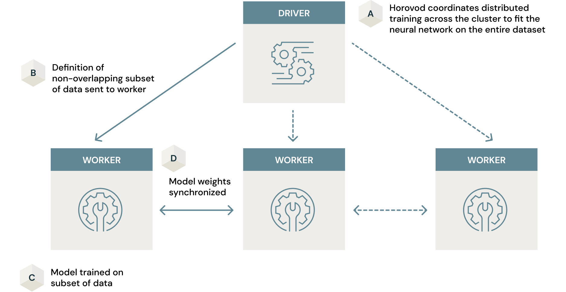
Parallelizing model training with Horovod

As we saw in the previous section, Hyperopt leverages Spark to distribute hyperparameter search by training multiple models with different hyperparameter combinations, in parallel. The training of each model takes place in a single machine. Distributed model training is yet another way in which distributed processing with Spark can make the training process more efficient. Here, a single model is trained across many machines in the cluster.

If the training dataset is large, it could be yet another bottleneck for training a production ready similarity model. Some approaches to this include training the model only on a subset of the data on a single machine. This comes at the cost of the final model being sub-optimal. However, with Spark and Horovod, an open-source framework for parallelizing the model training process across a cluster, this problem can be solved. Horovod, in conjunction with Spark, provides a data-parallel approach to model training on large-scale datasets with minimal code changes. Here, models are trained in parallel in each node in the cluster once definitions of subsets of data are passed, to learn weights of the neural network. These weights are synchronized across the cluster resulting in the final model. Ultimately, you end up with a highly optimized model trained on the entire dataset within a fraction of the time you would spend on attempting to do this on a single machine. The article How (Not) To Scale Deep Learning in 6 Easy Steps goes into great detail on how to leverage distributed compute for deep learning. Again, Horovod is most effective when used on a GPU cluster. Otherwise the advantages of scaling model training across a cluster would not bring the desired efficiencies.

Handling large image datasets for model training is another important factor to consider. In this example, fashion MNIST is a very small dataset that does not strain the cluster at all. However, large image datasets are often seen in the enterprise and a use case may involve training a similarity model on such data. Here, Petastorm, a data caching library built with Deep learning in mind, will be very useful. The linked notebook will help you leverage this technology for your use case.

Deploying model and index

Once the final model with the optimal hyperparameters is trained, the process of deploying a similarity model is a nuanced one. This is because the model and the index need to be deployed together. However, with MLflow, this process is trivially simple. As mentioned before, recommendations are retrieved by querying the index of data with the embedding inferred from the query sample. This can be illustrated in a simplified manner as follows.

One of the key advantages of this approach is that there is no need to retrain the model as new image data is received. Embeddings can be generated with the model and added to the ANN index for querying. Since the original image data is in the Delta format, any increments to the table will be recorded in the Delta transaction log. This ensures reproducibility of the entire data ingestion process.

In MLflow, there are numerous model flavors for popular (and even obscure) ML frameworks to enable easy packaging of models for serving. In practice, there are numerous instances where a trained model has to be deployed with pre and/or post processing logic, as in the case of the query-able similarity model and ANN index. Here we can use the mlflow.pyfunc module to create a custom `recommender model` class (named TfsimWrapper in this case ) to encapsulate the inference and lookup logic. This link provides detailed documentation on how this could be done.

```
import mlflow.pyfunc
class TfsimWrapper(mlflow.pyfunc.PythonModel):
    """ model input is a single row, single column pandas dataframe with base64 encoded byte string i.e. of the type bytes. Column name is 'input' in this case"""
    """ model output is a pandas dataframe where each row(i.e.element since only one column) is a string  converted to hexadecimal that has to be converted back to bytes and then a numpy array using np.frombuffer(...) and reshaped to (28, 28) and then visualized (if needed)"""
    
    def load_context(self, context):
      import tensorflow_similarity as tfsim
      from tensorflow_similarity.models import SimilarityModel
      from tensorflow.keras import models
      import pandas as pd
      import numpy as np
      
      
      self.tfsim_model = models.load_model(context.artifacts["tfsim_model"])
      self.tfsim_model.load_index(context.artifacts["tfsim_model"])

    def predict(self, context, model_input):
      from PIL import Image
      import base64
      import io

      image = np.array(Image.open(io.BytesIO(base64.b64decode(model_input["input"][0].encode()))))    
      #The model_input has to be of the form (1, 28, 28)
      image_reshaped = image.reshape(-1, 28, 28)/255.0
      images = np.array(self.tfsim_model.lookup(image_reshaped, k=5))
      image_dict = {}
      for i in range(5):
        image_dict[i] = images[0][i].data.tostring().hex()
        
      return pd.DataFrame.from_dict(image_dict, orient='index')

```

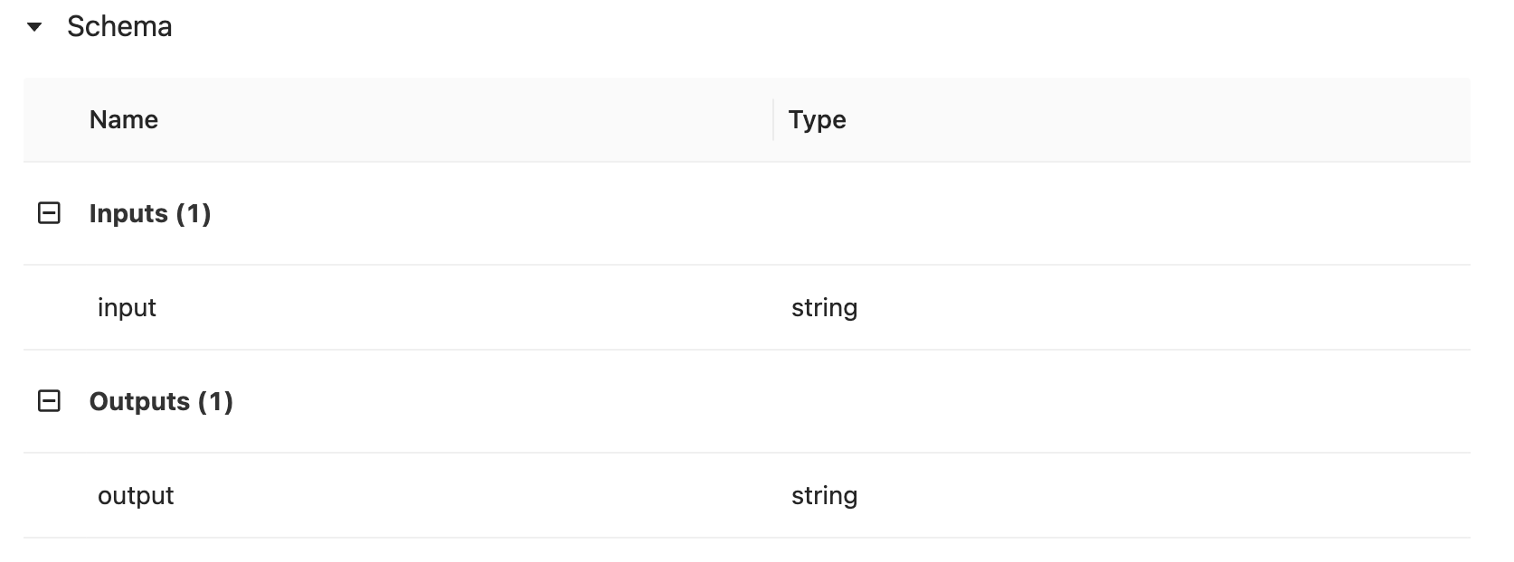
The model artifact can be logged, registered and deployed as a REST endpoint all within the same MLflow UI or by leveraging the MLflow API. In addition to this functionality, it is possible to define input and output schema as a model signature in the logging process to assist swift hand-off to deployment. This is handled automatically by including the following 3 lines of code

```
from mlflow.models.signature import infer_signature
signature = infer_signature(sample_image, loaded_model.predict(sample_image))
mlflow.pyfunc.log_model(artifact_path=mlflow_pyfunc_model_path, python_model=TfsimWrapper(), artifacts=artifacts,
        conda_env=conda_env, signature = signature)


```

Once the signature is inferred, data input output schema expectations will be indicated in the UI as follows.

Once the REST endpoint has been created, you can conveniently generate a bearer token by going to the user settings on the sliding panel on the left hand side of the workspace. With this bearer token, you can insert the automatically generated Python wrapper code for the REST endpoint in any end user facing application or internal process that relies on model inference.

The following function will help decode the JSON response from the REST call.

```
import numpy as np

def process_response_image(i):
“””response is the returned JSON object. We can loop through this object and return the reshaped numpy array for each recommended image which can then be rendered”””

  single_image_string = response[i]["0"]
  image_array = np.frombuffer(bytes.fromhex(single_image_string), dtype=np.float32)
  image_reshaped = np.reshape(image_array, (28,28))
  return image_reshaped

```

The code for a simple Streamlit application built to query this endpoint is available in the repository for this blog article. The following short recording shows the recommender in action.

Build your own with Databricks

Typically, the process of ingesting and formatting the data, model optimization, training at scale, and deploying a similarity model for recommendations is a novel and nuanced process for many. With the highly optimized managed Spark, Delta Lake, and MLflow foundations that Databricks provides, this process becomes simple and straightforward in the Lakehouse platform. Given that you can access managed compute clusters, the process of provisioning multiple GPUs is made seamless, with the entire process taking only several minutes. The notebook linked below walks you through the end to end process of building and deploying a similarity model in a detailed manner. We welcome you to try it, customize it in a manner that fits your needs, and build your own production-grade ML-based image recommendation system with Databricks.

Try the notebook.